(Pre-requisite)

(AST405) Lifetime data analysis

0 Parametric Regression Models

0.1 Linear Regression Model

Independent two-sample t-test

• Population A

  • Response $Y_1\sim \mathcal{N}({\mu }_1,{\sigma }^2)$

  • Random sample $\{y_{11},y_{12},\dots ,y_{1n_1}\}$

• Population B

  • Response $Y_2\sim \mathcal{N}({\mu }_2,{\sigma }^2)$

  • Random sample $\{y_{21},y_{22},\dots ,y_{2n_2}\}$

Objective $$H_0:{\mu }_1={\mu }_2$$

---

• Test statistic $$t=\frac{{\overline{y}}_1-{\overline{y}}_2}{se({\overline{y}}_1-{\overline{y}}_2)}=\frac{{\overline{y}}_1-{\overline{y}}_2}{s_p\sqrt{(1/n_1)+(1/n_2)}}\sim t_{n_1+n_2-2}$$

  • $s_p^2=\frac{(n_1-1)s_1^2+(n_2-1)s_2^2}{n_1+n_2-2}$

  • ${\overline{y}}_i=(1/n_i)\sum _{j=1}^{n_i}{y}_{ij}$

• $(1-\alpha )100\mathrm{\%}$ confidence interval for $({\mu }_1-{\mu }_2)$ $$({\overline{y}}_1-{\overline{y}}_2)\pm t_{n_1+n_2-2,1-\alpha /2}se({\overline{y}}_1-{\overline{y}}_2)$$

Melanoma mortality data

• Incidence of melanoma can be related to the amount of sunshine, equivalently to the latitude of the area

• Data were collected on malignant melanoma of the skin of white males during the period 1950–69 for each state of the US

• Data on mortality rate (per 10 million), 1965 population (in a million), latitude, longitude, and the whether the state borders on the ocean are recorded

---

Download mordat data

glimpse(mordat)

Rows: 49
Columns: 6
$ state     <chr> "Alabama", "Arizona", "Arkansas", "California", "Colorado", …
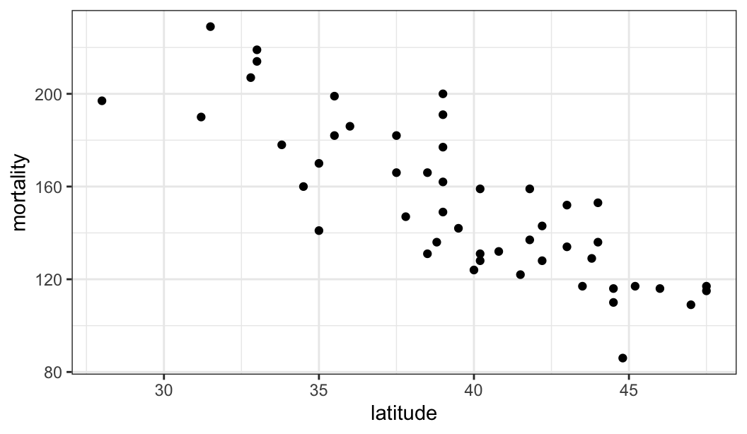
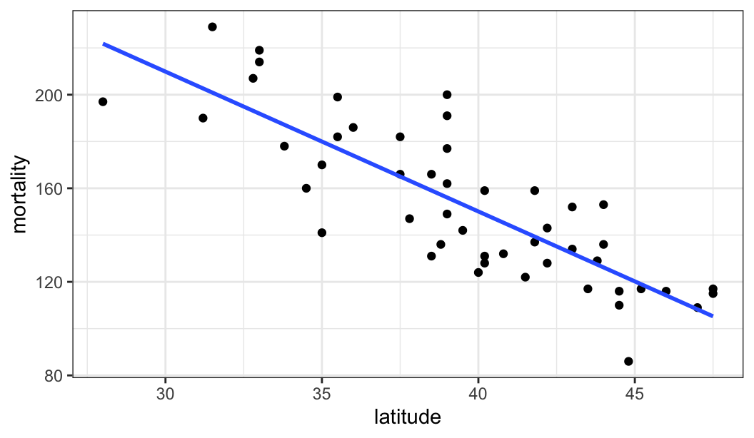
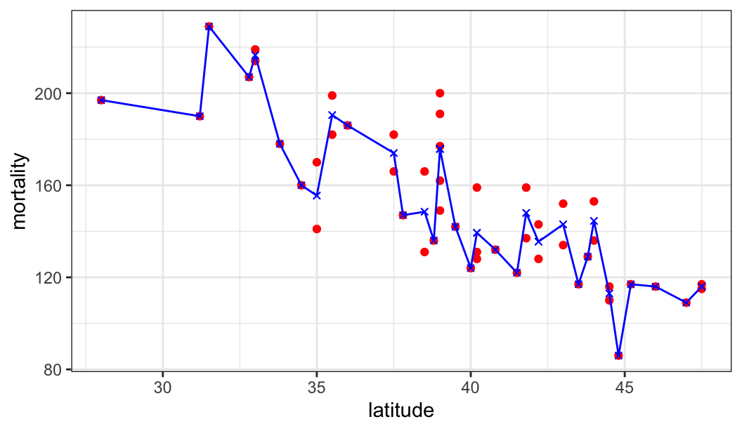
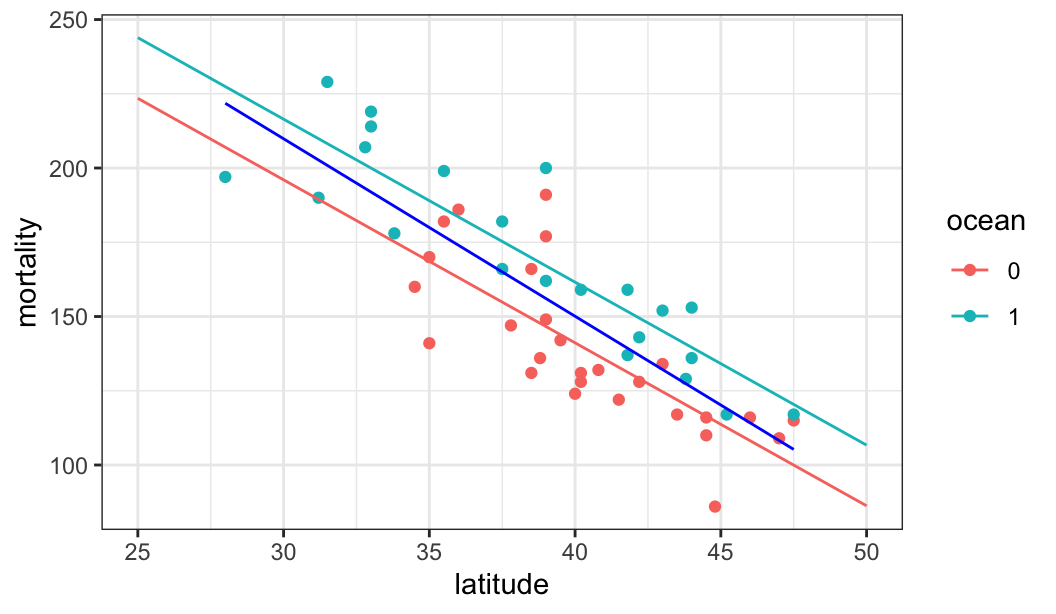
$ mortality <dbl> 219, 160, 170, 182, 149, 159, 200, 177, 197, 214, 116, 124, …
$ latitude  <dbl> 33.0, 34.5, 35.0, 37.5, 39.0, 41.8, 39.0, 39.0, 28.0, 33.0, …
$ longitude <dbl> 87.0, 112.0, 92.5, 119.5, 105.5, 72.8, 75.5, 77.0, 82.0, 83.…
$ pop       <dbl> 3.46, 1.61, 1.96, 18.60, 1.97, 2.83, 0.50, 0.76, 5.80, 4.36,…
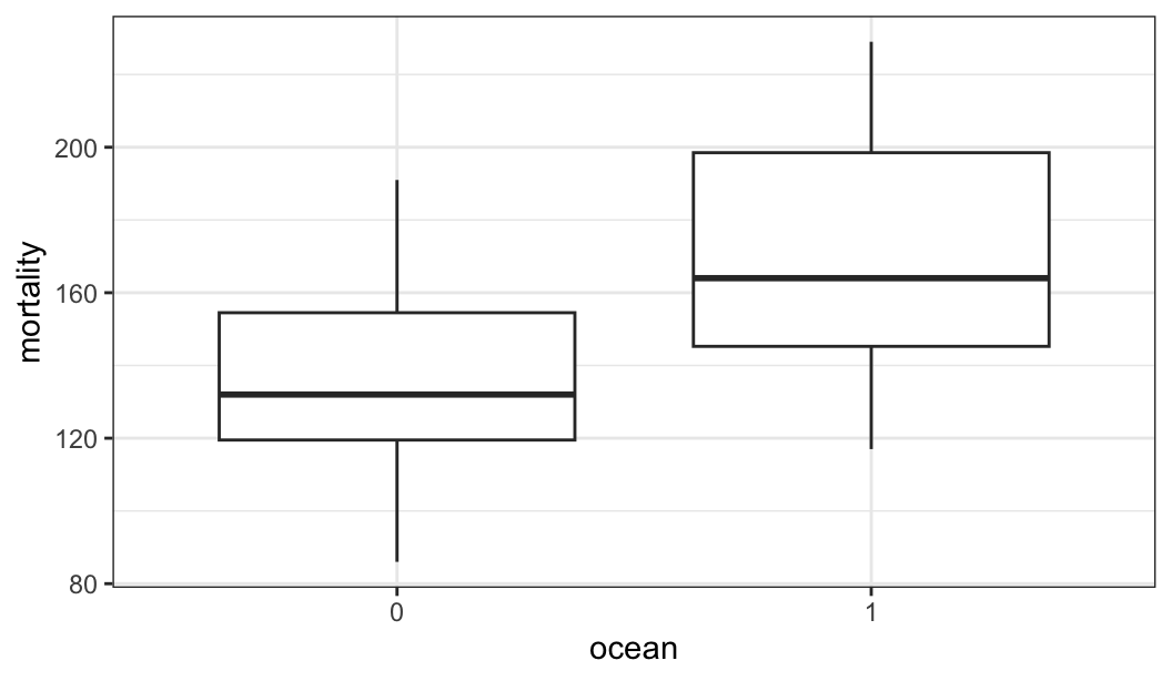
$ ocean     <fct> 1, 0, 0, 1, 0, 1, 1, 0, 1, 1, 0, 0, 0, 0, 0, 0, 1, 1, 1, 1, …

---

• For a state, does “contiguous to the ocean” (Yes or No) significantly affect melanoma mortality rate? $$\text{contiguous to ocean}=\{\begin{array}{ll}\text{Yes}\to & \text{ocean=1}\\ \text{No}\to & \text{ocean=0}\end{array}$$

---

Distribution of mortality rate by contiguous to ocean

Independent two-sample t-test

test1 <- t.test(mortality ~ ocean, var.equal = T, 
            data = mordat)
broom::tidy(test1) |>
  select(1:8) |> kable(digits = 3)

estimate	estimate1	estimate2	statistic	p.value	parameter	conf.low	conf.high
-31.487	138.741	170.227	-3.684	0.001	47	-48.68	-14.293

• “Contiguity to the ocean” has a significant effect on average mortality rate $(p<.001)$

Simple linear regression model

• Objective is to compare average mortality rate $(Y)$ between two group of states (ocean=0 or ocean=1)

$$\begin{array}{}\text{(1)}& E(Y|\text{ocean}=0)={\mu }_0\end{array}$$

$$\begin{array}{}\text{(2)}& E(Y|\text{ocean}=1)={\mu }_1\end{array}$$

• Expressing Equation 1 and Equation 2 in one equation $$\begin{array}{}\text{(3)}& E(Y|x_1)={\mu }_0+({\mu }_1-{\mu }_0)x_1\end{array}$$ where $$x_1=\{\begin{array}{ll}1& \text{if ocean=1}\\ 0& \text{if ocean=0}\end{array}$$

---

• Consider a model for mortality $(Y)$ on ocean $(x_1)$ $$\begin{array}{rl}E(Y|x_1)& ={\mu }_0+({\mu }_1-{\mu }_0)x_1\\ & ={\beta }_0+{\beta }_1{x}_1\end{array}$$ where $$\begin{array}{r}{\beta }_0={\mu }_0\text{and}{\beta }_1=({\mu }_1-{\mu }_0)\end{array}$$

• Comparison between two groups of states $$H_0:{\beta }_1=0\Rightarrow H_0:{\mu }_1={\mu }_2$$

---

• Another way of defining simple linear model, let $Y(x)$ be response corresponding to a subject with predictor $x$ and assume $$\begin{array}{r}(Y|x)=Y(x)\sim \mathcal{N}(\mu (x),{\sigma }^2)\end{array}$$
• Parametric regression model $$\begin{array}{rl}\mu (x)=E(Y|x)& ={\beta }_0+{\beta }_{1}x\\ V(Y|x)& ={\sigma }^2\end{array}$$

---

• Data $$\{(y_i,x_i),i=1,\dots ,n\}$$

• Assume $y$’s are independent and $$Y_i\sim \mathcal{N}(\mu (x_i),{\sigma }^2)$$

• Simple linear regression model

$$\begin{array}{rl}\mu (x)=E(Y|x)& ={\beta }_0+{\beta }_{1}x\\ V(Y|x)& ={\sigma }^2\end{array}$$

• Both maximum likelihood and ordinary least square methods can be used to estimate the parameters of linear regression models

Estimation of parameters

• Log-likelihood function $$\begin{array}{rl}\ell ({\beta }_0,{\beta }_1)& =\log \prod _{i=1}^n(1/\sigma )\varphi (\frac{y_i-\mu (x_i)}{\sigma })\\ & =-n\log \sigma +\sum _{i=1}^n\log \varphi (\frac{y_i-{\beta }_0-{\beta }_1{x}_i}{\sigma })\end{array}$$

• MLEs $$\begin{array}{r}({\hat{\beta }}_0,{\hat{\beta }}_1{)}^{\prime }={\arg max}_{\mathrm{\Theta }}\ell ({\beta }_0,{\beta }_1)\end{array}$$

---

• Estimating the effect of “contiguous to ocean” $(x_1)$ on mortality rate $(Y)$ using simple linear regression model $$E(Y|x_1)={\beta }_0+{\beta }_1{x}_1$$

---

• Fitting a linear model for mortality with “contiguous to ocean” as the only predictor

mod_oc <- lm(mortality ~ ocean, data = mordat)
tbl_regression(mod_oc, intercept = T)

Characteristic	Beta	95% CI1	p-value
(Intercept)	139	127, 150	<0.001
ocean
0	—	—
1	31	14, 49	<0.001
1 CI = Confidence Interval

• “Contiguity to the ocean” has a significant effect on average mortality rate $(p<.001)$

---

• Fitted model $$\begin{array}{rl}E(Y|x_1)& =138.741+31.487x_1=\{\begin{array}{ll}138.741& \text{if }{x}_1=0\\ 170.227& \text{if }{x}_1=1\end{array}\end{array}$$

• Inland states (ocean=0) are expected to have about 31 fewer melanoma deaths (per 10 million population) compared to other states

t-test and simple linear regression model

• For binary predictors, inference based on independent two-sample t-test and simple linear regression mode are similar

• The method of simple linear regression model for binary predictor can also be used for continuous predictor

Simple linear regression model with a continuous predictor

• Model I: a model for mortality $(Y)$ on latitude $(x_2)$ $$\begin{array}{rl}E(Y|x_2)& ={\beta }_0+{\beta }_2{x}_2\\ V(Y|x_2)& ={\sigma }^2\end{array}$$

---

Scatter plot of mortality vs latitude

---

mod_l1 <- lm(mortality ~ latitude, data = mordat)
tbl_regression(mod_l1, intercept = T)

Characteristic	Beta	95% CI1	p-value
(Intercept)	389	341, 437	<0.001
latitude	-6.0	-7.2, -4.8	<0.001
1 CI = Confidence Interval

• Latitude has a significant effect on the melanoma mortality rate

• For one-degree increase in latitude (i.e., moving toward the north), melanoma mortality rate decrease by 6 deaths per 10 million population

---

ANOVA table for Model I

tidy(aov(mod_l1)) |> kable(digits = 3)

term	df	sumsq	meansq	statistic	p.value
latitude	1	36464.20	36464.200	99.797	0
Residuals	47	17173.06	365.384	NA	NA

---

Fit of Model I

Another fit of the model “Mortality on latitude”

• Model I: A model for mortality on latitude $(x_2)$ $$\begin{array}{r}E(Y|x_2)={\beta }_0+{\beta }_2{x}_2\end{array}$$

• Model II: A model for mortality on latitude $(x)$ $$\begin{array}{r}E(Y|x)={\beta }_0+{\beta }_{x}x\end{array}$$

---

mod_l2 <- lm(mortality ~ latitudef, 
             data = mordat %>% 
                 mutate(latitudef = factor(latitude)))
tbl_regression(mod_l2, intercept = T)

Characteristic	Beta	95% CI1	p-value
(Intercept)	197	163, 231	<0.001
latitudef
28	—	—
31.2	-7.0	-55, 41	0.8
31.5	32	-16, 80	0.2
32.8	10	-38, 58	0.7
33	20	-22, 61	0.3
33.8	-19	-67, 29	0.4
34.5	-37	-85, 11	0.12
35	-42	-83, -0.35	0.048
35.5	-6.5	-48, 35	0.7
36	-11	-59, 37	0.6
37.5	-23	-64, 18	0.3
37.8	-50	-98, -2.5	0.040
38.5	-49	-90, -7.4	0.024
38.8	-61	-109, -13	0.015
39	-21	-58, 16	0.2
39.5	-55	-103, -7.5	0.026
40	-73	-121, -25	0.005
40.2	-58	-96, -19	0.006
40.8	-65	-113, -17	0.010
41.5	-75	-123, -27	0.004
41.8	-49	-90, -7.9	0.022
42.2	-62	-103, -20	0.006
43	-54	-95, -13	0.013
43.5	-80	-128, -32	0.002
43.8	-68	-116, -20	0.008
44	-53	-94, -11	0.015
44.5	-84	-125, -43	<0.001
44.8	-111	-159, -63	<0.001
45.2	-80	-128, -32	0.002
46	-81	-129, -33	0.002
47	-88	-136, -40	0.001
47.5	-81	-122, -40	<0.001
1 CI = Confidence Interval

---

ANOVA table for Model II

tidy(aov(mod_l2)) |> kable(digits = 4)

term	df	sumsq	meansq	statistic	p.value
latitudef	31	49326.799	1591.1871	6.2755	1e-04
Residuals	17	4310.467	253.5569	NA	NA

---

Comparison between Model I and Model II (LRT)

tidy(anova(mod_l1, mod_l2)) |> kable(digits = 3)

term	df.residual	rss	df	sumsq	statistic	p.value
mortality ~ latitude	47	17173.065	NA	NA	NA	NA
mortality ~ latitudef	17	4310.467	30	12862.6	1.691	0.128

---

Fit of Model II

---

Comparison between the fits of Models I and II

---

Residuals of Models I and II

---

Which model (I or II) do you prefer for analyzing the data?

---

Estimate and corresponding confidence intervals obtained using Models I and II

Multiple linear regression model

• A model for mortality rate $(Y)$ on ocean $(x_1)$ and latitude $(x_2)$ $$\begin{array}{rl}E(Y|x_1,x_2)& ={\beta }_0+{\beta }_1{x}_1+{\beta }_2{x}_2\\ V(Y|x_1,x_2)& ={\sigma }^2\end{array}$$

---

mod_2 <- lm(mortality ~ ocean + latitude, 
            data = mordat)
tbl_regression(mod_2, intercept = T)

Characteristic	Beta	95% CI1	p-value
(Intercept)	361	317, 404	<0.001
ocean
0	—	—
1	20	11, 30	<0.001
latitude	-5.5	-6.5, -4.4	<0.001
1 CI = Confidence Interval

• Both contiguity to ocean and latitude have significant effects on the mortality rate

---

• On average, inland states have about 20 fewer melanoma deaths compared to other states provided latitude is fixed

• For one-degree increase of latitude, the average mortality rate decrease by 5 deaths per 10 million population provided contiguity to the ocean is fixed

---

Comparison of the fits of the simple (blue line) and multiple linear regression models for mortality

0.2 Logistic Regression Model

Contingency table

• Data obtained from different types of study designs (e.g., prospective, retrospective, and cross-sectional) can be expressed in such contingency table to examine the exposure-disease relationship

	Disease
Exposure	Yes	No	Total
Yes	a	b	n_1
No	c	d	n_2
Total	m_1	m_2	n

Prospective study design

• Let $Y_1$ and $Y_2$ be the number of exposed and non-exposed diseased subjects, which follow two independent binomial distributions $$Y_1\sim B(n_1,p_1)\text{and}{Y}_2\sim B(n_2,p_2)$$

  • $p_1=Pr(D=1|E=1)$

  • $p_2=Pr(D=1|E=0)$

• Estimate of model parameters $$\begin{array}{r}{\hat{p}}_1=(a/n_1)and{\hat{p}}_2=(c/n_2)\end{array}$$

---

• Risk difference $$\begin{array}{rl}RD& =p_1-p_2\\ \widehat{RD}& ={\hat{p}}_1-{\hat{p}}_2\\ se(\widehat{RD})& =[({\hat{p}}_1{\hat{q}}_1/n_1)+({\hat{p}}_2{\hat{q}}_2/n_2){]}^{1/2}\end{array}$$

---

• Risk ratio $$\begin{array}{rl}RR& =(p_1/p_2)\\ \widehat{RR}& =({\hat{p}}_1/{\hat{p}}_2)\\ se(\log \widehat{RR})& =[\frac{{\hat{q}}_1}{n_1{\hat{p}}_1}+\frac{{\hat{q}}_2}{n_2{\hat{p}}_2}{]}^{1/2}\end{array}$$

---

• Odds $\iff$ probability $$o(x)=\frac{p(x)}{1-p(x)}\Rightarrow p(x)=\frac{o(x)}{1+o(x)}$$

• Odds ratio $$\begin{array}{rl}OR& =\frac{p_1/q_1}{p_2/q_2}\\ \widehat{OR}& =\frac{{\hat{p}}_1/{\hat{q}}_1}{{\hat{p}}_2/{\hat{q}}_2}=\frac{ad}{bc}\\ se(\log \widehat{OR})& =[\frac{1}{a}+\frac{1}{b}+\frac{1}{c}+\frac{1}{d}{]}^{1/2}\end{array}$$

Case-control study design

• Let $Y_1$ and $Y_2$ be the number of exposed subjects in case and control groups, respectively, following two independent binomial distributions $$Y_1\sim B(m_1,p_1)\text{and}{Y}_2\sim B(m_2,p_2)$$

  • $p_1=Pr(E=1|D=1)$

  • $p_2=Pr(E=1|D=0)$

• Estimate of parameters $${\hat{p}}_1=(a/m_1)\text{and}{\hat{p}}_2=(b/m_2)$$

---

• Odds ratio $$\begin{array}{rl}OR& =\frac{p_1/q_1}{p_2/q_2}\\ \widehat{OR}& =\frac{{\hat{p}}_1/{\hat{q}}_1}{{\hat{p}}_2/{\hat{q}}_2}=\frac{ad}{bc}\end{array}$$

  • Disease-odds-ratio = Exposure-odds-ratio

  • For case-control study, the RR can be approximated by OR if the disease is rare

Cross-sectional study

• Data of dichotomous disease-exposure study can be considered as an outcome of $n$ tosses of a four-faced dye with the faces $$\{ED\},\{E\overline{D}\},\{\overline{E}D\},\{\overline{E}\overline{D}\}$$

  • Estimators of odds ratio $$\widehat{OR}=\frac{ad}{bc}$$

  • Multinomial distribution is associated with the outcome of a cross-sectional study

Western Collaborative Group Study (WCGS)

• A large epidemiological study designed to investigate the association between the Type-A behavior pattern and coronary heart disease (CHD)

• Type-A behavior is composed of competitiveness, excessive drive, and an enhanced sense of time urgency

• Download wcgs data

---

head(wcgs) |> select(1:10) |> kable()

age	arcus	behpat	bmi	chd69	chol	dbp	dibpat	height	id
50	1	A1	31.32101	0	249	90	Type A	67	2343
51	0	A1	25.32858	0	194	74	Type A	73	3656
59	1	A1	28.69388	0	258	94	Type A	70	3526
51	1	A1	22.14871	0	173	80	Type A	69	22057
44	0	A1	22.31303	0	214	80	Type A	71	12927
47	0	A1	27.11768	0	206	76	Type A	64	16029

• Outcome: chd69
• Exposure: dibpat

---

	CHD
dibpat	1	0	total	$\hat{p}$	$\hat{o}$
Type A	177	1411	1588	0.111	0.125
Type B	78	1486	1564	0.050	0.053

• $\widehat{RD}=0.111-0.05=0.061$

• Subjects with Type-A behavior have about 6.1 % higher risk of developing CHD compared with others

---

	CHD
dibpat	1	0	total	$\hat{p}$	$\hat{o}$
Type A	177	1411	1588	0.111	0.125
Type B	78	1486	1564	0.050	0.053

• $\widehat{RR}=(0.111/0.05)=2.22$

• The risk of developing CHD for Type-A subjects is about 2.2 times the risk for Type-B subjects

• In other words, the risk of developing CHD is about $122$% higher for Type-A subjects compared to Type-B subjects

---

	CHD
dibpat	1	0	total	$\hat{p}$	$\hat{o}$
Type A	177	1411	1588	0.111	0.125
Type B	78	1486	1564	0.050	0.053

• $\widehat{OR}=(0.125/0.053)=2.358$

• The odds of developing CHD for Type-A subjects is about 2.4 times that the risk for Type-B subjects

• In other words, the odds of developing CHD is about $136$% higher for Type-A subjects compared to Type-B subjects

---

$$\begin{array}{rl}\widehat{RD}\pm se(\widehat{RD})& =0.061\pm 0.01\\ \log \widehat{RR}\pm se(\log \widehat{RR})& =0.798\pm 0.131\\ \log \widehat{OR}\pm se(\log \widehat{OR})& =0.858\pm 0.141\end{array}$$

• Obtain confidence intervals for RD, RR, and OR

Regression model for binary response

• Let $Y(x)$ be binary response obtained from a subject with predictor value $x$ and assume $$Y(x)\sim B(1,p(x))$$ where $$p(x)=Pr(Y(x)=1)=Pr(Y=1|x)=E(Y|x)$$

Regression models for $p(x)$

• Assume $Y(x)\sim B(1,p(x))$ $$\begin{array}{}\text{(Model I)}& p(x)={\beta }_0+{\beta }_{1}x\end{array}$$

  • $-\mathrm{\infty }<p(x)<\mathrm{\infty }$

  • Linear probability model

---

• Assume $Y(x)\sim B(1,p(x))$ $$\begin{array}{}\text{(Model II)}& \log p(x)={\beta }_0+{\beta }_{1}x\Rightarrow p(x)=\exp ({\beta }_0+{\beta }_{1}x)\end{array}$$

  • $0<p(x)<\mathrm{\infty }$

  • Log-binomial model

---

• Assume $Y(x)\sim B(1,p(x))$ $$\begin{array}{rl}\text{logit}p(x)& =\log \frac{p(x)}{1-p(x)}={\beta }_0+{\beta }_{1}x\\ \text{(Model III)}& p(x)& =\frac{\exp ({\beta }_0+{\beta }_{1}x)}{1+\exp ({\beta }_0+{\beta }_{1}x)}\end{array}$$

  • $0<p(x)<1$

  • Logistic regression model (related to the distribution function of logistic distribution)

---

• Assume $Y(x)\sim B(1,p(x))$ $$\begin{array}{rl}{\mathrm{\Phi }}^{-1}(p(x))& ={\beta }_0+{\beta }_{1}x\\ \text{(Model IV)}& p(x)& =\mathrm{\Phi }({\beta }_0+{\beta }_{1}x)\end{array}$$

  • $0<p(x)<1$

  • Probit regression model

---

• Assume $Y(x)\sim B(1,p(x))$ $$\begin{array}{rl}\log [-\log (1-p(x))]& ={\beta }_0+{\beta }_{1}x\\ \text{(Model V)}& p(x)& =1-\exp [-e^{{\beta }_0+{\beta }_{1}x}]\end{array}$$

  • $0<p(x)<1$

  • Regression model with complementary log-log link (related to the distribution function of extreme-value distribution)

---

Model I: $p(x)={\beta }_0+{\beta }_{1}x$

• Probability of developing CHD among subjects with Type-A $(x=1)$ and Type-B behavior $(x=0)$ $$\begin{array}{rl}p(1)& =P(Y=1|x=1)={\beta }_0+{\beta }_1\\ p(0)& =P(Y=1|x=0)={\beta }_0\end{array}$$

  • Effect of behavior type on CHD $$RD=p(1)-p(0)={\beta }_1$$

---

Data $$\{(y_i,x_i),i=1,\dots ,n\}$$

$y$’s are independent and assume $$Y_i\sim B(1,p(x_i))$$

• Linear probability model $$p(x_i)={\beta }_0+{\beta }_1{x}_i$$

---

Log-likelihood function $$\begin{array}{rl}\ell ({\beta }_0,{\beta }_1)& =\log \prod _{i=1}^n{y}_i^{p(x_i)}(1-y_i{)}^{1-p(x_i)}\\ & =\sum _{i=1}^n\{({\beta }_0+{\beta }_1{x}_i)\log y_i+(1-{\beta }_0-{\beta }_1{x}_i)\log (1-y_i)\}\end{array}$$

• MLEs $$\begin{array}{r}({\hat{\beta }}_0,{\hat{\beta }}_1{)}^{\prime }={\arg max}_{\mathrm{\Theta }}\ell ({\beta }_0,{\beta }_1)\end{array}$$

glm() funciton

R function glm() is used to fit a generalized linear model

glm(formula, data, family)

• family specifies the distribution of response and link function, which can be either a string or a function, and commonly used family and link function in glm()

  • binomial("logit") $\to$ binomial distribution and logit link function

  • binomial("log") $\to$ binomial distribution and log link function

  • gaussian("identity") $\to$ Gaussian distribution and identity link function

  • poisson("log") $\to$ Poisson distribution and log link function

Model I: $p(x)={\beta }_0+{\beta }_{1}x$

bmod_1 <- glm(chd69 ~ dibpat, family = binomial("identity"), 
              data = wcgs)
tbl_regression(bmod_1, intercept = T)

Characteristic	Beta	95% CI1	p-value
(Intercept)	0.05	0.04, 0.06	<0.001
dibpat
Type B	—	—
Type A	0.06	0.04, 0.08	<0.001
1 CI = Confidence Interval

• Since response chd69 is a binary variable and regression function is assumed to be identically linked with the parameter of the response distribution, a binomial("identity") is used as family

• Effect of behavior type on CHD $$\widehat{RD}={\hat{\beta }}_1=0.062$$

Model II: $\log p(x)={\beta }_0+{\beta }_{1}x$

• Probability of developing CHD among subjects with Type-A $(x=1)$ and Type-B $(x=0)$ behavior $$\begin{array}{rl}p(1)& =P(Y=1|x=1)=\exp ({\beta }_0+{\beta }_1)\\ p(0)& =P(Y=1|x=0)=\exp ({\beta }_0)\end{array}$$

• Effect of Type-A behavior $$RR=\frac{p(1)}{p(0)}=\exp ({\beta }_1)\Rightarrow \log RR={\beta }_1$$

---

Log-likelihood function $$\begin{array}{rl}\ell ({\beta }_0,{\beta }_1)& =\log \prod _{i=1}^n{y}_i^{p(x_i)}(1-y_i{)}^{1-p(x_i)}\\ & =\sum _{i=1}^n\{\exp ({\beta }_0+{\beta }_1{x}_i)\log y_i+[1-\exp ({\beta }_0+{\beta }_1{x}_i)]\log (1-y_i)\}\end{array}$$

• MLEs $$\begin{array}{r}({\hat{\beta }}_0,{\hat{\beta }}_1{)}^{\prime }={\arg max}_{\mathrm{\Theta }}\ell ({\beta }_0,{\beta }_1)\end{array}$$

---

bmod_2 <- glm(chd69 ~ dibpat, family = binomial("log"), 
              data = wcgs)
tbl_regression(bmod_2, intercept = T)

Characteristic	log(RR)1	95% CI1	p-value
(Intercept)	-3.0	-3.2, -2.8	<0.001
dibpat
Type B	—	—
Type A	0.80	0.55, 1.1	<0.001
1 RR = Relative Risk, CI = Confidence Interval

• Since response chd69 is a binary variable and regression function is assumed to be linked with the log-transformed parameter of the response distribution, a binomial("log") is used as family

• Effect of behavior type on CHD $$\log \widehat{RR}={\hat{\beta }}_1=0.804\Rightarrow \widehat{RR}=\exp ({\hat{\beta }}_1)=2.235$$

Model III: $\text{logit}p(x)={\beta }_0+{\beta }_{1}x$

• Probability of developing CHD among subjects with Type-A $(x=1)$ and Type-B $(x=0)$ behavior $$\begin{array}{rl}p(1)& =P(Y=1|x=1)=\frac{\exp ({\beta }_0+{\beta }_1)}{1+\exp ({\beta }_0+{\beta }_1)}\\ p(0)& =P(Y=1|x=0)=\frac{\exp ({\beta }_0)}{1+\exp ({\beta }_0)}\end{array}$$

---

• Effect of behavior type $$\begin{array}{rl}& OR=\frac{p(1)/[1-p(1)]}{p(0)/[1-p(0)]}=\frac{\exp ({\beta }_0+{\beta }_1)}{\exp ({\beta }_0)}=\exp ({\beta }_1)\\ \Rightarrow & \log OR={\beta }_1\end{array}$$

---

Log-likelihood function $$\begin{array}{rl}\ell ({\beta }_0,{\beta }_1)& =\log \prod _{i=1}^n{y}_i^{p(x_i)}(1-y_i{)}^{1-p(x_i)}\\ & =\sum _{i=1}^n\{\frac{\exp ({\beta }_0+{\beta }_1{x}_i)}{1+\exp ({\beta }_0+{\beta }_1{x}_i)}\log y_i+\frac{\log (1-y_i)}{1+\exp ({\beta }_0+{\beta }_1{x}_i)}\}\end{array}$$

• MLEs $$\begin{array}{r}({\hat{\beta }}_0,{\hat{\beta }}_1{)}^{\prime }={\arg max}_{\mathrm{\Theta }}\ell ({\beta }_0,{\beta }_1)\end{array}$$

---

bmod_3 <- glm(chd69 ~ dibpat, family = binomial("logit"), 
              data = wcgs)
tbl_regression(bmod_3, intercept = T)

Characteristic	log(OR)1	95% CI1	p-value
(Intercept)	-2.9	-3.2, -2.7	<0.001
dibpat
Type B	—	—
Type A	0.87	0.60, 1.2	<0.001
1 OR = Odds Ratio, CI = Confidence Interval

• Since response chd69 is a binary variable and the regression function is assumed to be linked with a logit-transformed parameter of the response distribution, a binomial("logit") is used as family

• Effect of behavior type on CHD $$\log \widehat{OR}={\hat{\beta }}_1=0.871\Rightarrow \widehat{OR}=\exp ({\hat{\beta }}_1)=2.39$$

Binary response and continuous predictor

• Effect of age $(x_2)$ on CHD (Model I) $$p(x)={\beta }_0+{\beta }_1{x}_2$$

mod_1a <- glm(chd69 ~ age, family = binomial("identity"), 
              data = wcgs)
tbl_regression(mod_1a, intercept = T)

Characteristic	Beta	95% CI1	p-value
(Intercept)	-0.17	-0.25, -0.10	<0.001
age	0.01	0.00, 0.01	<0.001
1 CI = Confidence Interval

• Age has a significant effect on CHD, and for an increase of 10 years, risk of developing CHD increase by 0.055

---

• What is the risk of developing CHD for a subject of age 45?

predict.glm(mod_1a, newdata = list(age = 45), 
            type = "response")

         1 
0.07393095 

---

• Predicting linear predictor for a subject of age 45

predict.glm(mod_1a, newdata = list(age = 45), 
            type = "link")

         1 
0.07393095 

Binary response and continuous predictor

• Effect of age $(x_2)$ on CHD (Model II) $$\log p(x)={\beta }_0+{\beta }_1{x}_2$$

mod_2a <- glm(chd69 ~ age, family = binomial("log"), 
              data = wcgs)
tbl_regression(mod_2a, intercept = T)

Characteristic	log(RR)1	95% CI1	p-value
(Intercept)	-5.7	-6.7, -4.8	<0.001
age	0.07	0.05, 0.09	<0.001
1 RR = Relative Risk, CI = Confidence Interval

• Age has a significant effect on CHD, and the risk of developing CHD for a subject John is 1.07 $(=e^{0.068})$ times that of a subject who is one year younger than John

• For one year increase of age, the risk of developing CHD is increased by 7%

---

What is the risk of developing CHD for a subject of age 45?

predict.glm(mod_2a, newdata = list(age = 45), 
            type = "response")

         1 
0.06891375 

Predicting linear predictor for a subject of age 45

predict.glm(mod_2a, newdata = list(age = 45), 
            type = "link")

      1 
-2.6749 

Binary response and continuous predictor

Effect of age $(x_2)$ on CHD (Model III) $$\text{logit}p(x)={\beta }_0+{\beta }_1{x}_2$$

mod_3a <- glm(chd69 ~ age, family = binomial("logit"), 
              data = wcgs)
tbl_regression(mod_3a, intercept = T)

Characteristic	log(OR)1	95% CI1	p-value
(Intercept)	-6.0	-7.1, -4.9	<0.001
age	0.07	0.05, 0.10	<0.001
1 OR = Odds Ratio, CI = Confidence Interval

• Age has a significant effect on CHD, and the odds of developing CHD for a subject John is 1.078 $(=e^{0.075})$ times that of a subject who is one year younger than John

• For one year increase of age, the odds of developing CHD is increased by 7.8%

---

• What is the risk of developing CHD for a subject of age 45?

predict.glm(mod_3a, newdata = list(age = 45), 
            type = "response")

         1 
0.06913919 

• Predicting linear predictor for a subject of age 45

predict.glm(mod_3a, newdata = list(age = 45), 
            type = "link")

        1 
-2.599988 

---

Comparisons among the fits of the regression models I, II, and III with age as the predictor

Multiple logistic regression models

• Model for binary response CHD $(Y)$ with predictors behavior type $(x_1)$ and $(x_2)$ $$p(x)={\beta }_0+{\beta }_1{x}_1+{\beta }_2{x}_2$$

mod_1b <- glm(chd69 ~ dibpat + age, family = binomial("identity"),
              data = wcgs)
tbl_regression(mod_1b, intercept = T)

Characteristic	Beta	95% CI1	p-value
(Intercept)	-0.15	-0.22, -0.08	<0.001
dibpat
Type B	—	—
Type A	0.05	0.03, 0.07	<0.001
age	0.00	0.00, 0.01	<0.001
1 CI = Confidence Interval

• The effect of behavior type on CHD is constant over age, and the effect of age is constant over two levels of behavior types

---

• Estimated risks for the subjects John (age 40, Type-A), Allan (age 40, Type-A), Tom (age 50, Type-B), and Steve (age 40, Type-B)

# A tibble: 4 × 3
  subject   age dibpat
* <chr>   <dbl> <chr> 
1 John       40 Type A
2 Allan      40 Type B
3 Tom        50 Type A
4 Steve      50 Type B

---

predict.glm(mod_1b, newdata = ndat1b,
            type = "response")

      John      Allan        Tom      Steve 
0.07782783 0.02795346 0.12257767 0.07270330 

• Estimate of the effect of behavior type in terms of RD, RR, and OR from the pairs John-Allan and Tom-Steve

---

Estimate of RD, OR, and RR for assessing the effects of behavior type on CHD at different values of age using linear probability model

---

• Model for binary response CHD $(Y)$ with predictors behavior type $(x_1)$ and $(x_2)$ $$\log p(x)={\beta }_0+{\beta }_1{x}_1+{\beta }_2{x}_2$$

mod_2b <- glm(chd69 ~ dibpat + age, family = binomial("log"),
              data = wcgs)
tbl_regression(mod_2b, intercept = T)

Characteristic	log(RR)1	95% CI1	p-value
(Intercept)	-5.9	-6.8, -4.9	<0.001
dibpat
Type B	—	—
Type A	0.74	0.48, 1.0	<0.001
age	0.06	0.04, 0.08	<0.001
1 RR = Relative Risk, CI = Confidence Interval

• The Effect of behavior type on CHD is constant over age, and the effect of age is constant over two levels of behavior types

---

ndat1b

# A tibble: 4 × 3
  subject   age dibpat
* <chr>   <dbl> <chr> 
1 John       40 Type A
2 Allan      40 Type B
3 Tom        50 Type A
4 Steve      50 Type B

predict.glm(mod_2b, newdata = ndat1b,
            type = "response")

      John      Allan        Tom      Steve 
0.06893735 0.03298930 0.12762092 0.06107175 

• Estimate of the effect of behavior type in terms of RD, RR, and OR from the pairs John-Allan and Tom-Steve

---

Estimate of RD, OR, and RR for assessing the effects of behavior type on CHD at different values of age using log-binomial model

---

• Model for binary response CHD $(Y)$ with predictors behavior type $(x_1)$ and $(x_2)$ $$\text{logit}p(x)={\beta }_0+{\beta }_1{x}_1+{\beta }_2{x}_2$$

mod_3b <- glm(chd69 ~ dibpat + age, family = binomial("logit"),
              data = wcgs)
tbl_regression(mod_3b, intercept = T)

Characteristic	log(OR)1	95% CI1	p-value
(Intercept)	-6.2	-7.3, -5.1	<0.001
dibpat
Type B	—	—
Type A	0.81	0.53, 1.1	<0.001
age	0.07	0.05, 0.09	<0.001
1 OR = Odds Ratio, CI = Confidence Interval

• The effect of behavior type on CHD is constant over age, and the effect of age is constant over two levels of behavior types

---

ndat1b

# A tibble: 4 × 3
  subject   age dibpat
* <chr>   <dbl> <chr> 
1 John       40 Type A
2 Allan      40 Type B
3 Tom        50 Type A
4 Steve      50 Type B

predict.glm(mod_3b, newdata = ndat1b,
            type = "response")

      John      Allan        Tom      Steve 
0.06885560 0.03198807 0.12857668 0.06185677 

• Estimate of the effect of behavior type in terms of RD, RR, and OR from the pairs John-Allan and Tom-Steve

---

Estimate of RD, OR, and RR for assessing the effects of behavior type on CHD at different values of age using logistic regression model

Interaction

• Consider a model for binary response CHD with three predictors “behavior type” $(x_1)$, “age” $(x_2)$, and “arcus senilis” $(x_3)$

  • age $(x_2)$ is a continuous predictor

  • behavior type $(x_1)$ and arcus senilis $(x_2)$ are binary predictor

$$\begin{array}{rl}{x}_1& =\{\begin{array}{ll}1& \text{‘Type-A‘}\\ 0& \text{‘Type-B‘}\end{array}\\ x_3& =\{\begin{array}{ll}1& \text{arcus senilis = Yes}\\ 0& \text{arcus senilis = No}\end{array}\end{array}$$

---

• Logistic regression model without the interaction term $$\begin{array}{r}\text{logit}p(x)={\beta }_0+{\beta }_1{x}_1+{\beta }_2{x}_2+{\beta }_3{x}_3\end{array}$$

  • $\widehat{OR}=\exp ({\beta }_2)\to$ Effect of behavior type on the odds of CHD after adjusting for age and arcus senilis

---

mod_3c <- glm(chd69 ~  dibpat + age + arcus, 
              data = wcgs, family = binomial("logit"))
tbl_regression(mod_3c, intercept = T)

Characteristic	log(OR)1	95% CI1	p-value
(Intercept)	-6.0	-7.1, -5.0	<0.001
dibpat
Type B	—	—
Type A	0.80	0.52, 1.1	<0.001
age	0.06	0.04, 0.09	<0.001
arcus
0	—	—
1	0.32	0.04, 0.59	0.023
1 OR = Odds Ratio, CI = Confidence Interval

• $\widehat{OR}=2.225=\exp (0.8)$

• Odds of developing CHD for a subject with Type-A behavior is 2.2 times than that of a subject with Type-B behavior provided age and arcus senilis is constant

---

---

• Logistic regression model with an interaction term between “behavior type” and “arcus senilis” $$\begin{array}{rl}\text{logit}p(x)& ={\beta }_0+{\beta }_1{x}_1+{\beta }_2{x}_2+{\beta }_3{x}_3+\theta x_1{x}_3\\ & =\{\begin{array}{ll}({\beta }_0+{\beta }_3)+({\beta }_1+\theta )x_1+{\beta }_2{x}_2& \text{for }{x}_3=1\\ {\beta }_0+{\beta }_1{x}_1+{\beta }_2{x}_2& \text{for }{x}_3=0\end{array}\end{array}$$

  • If $\theta \ne 0\to$ Association between behavior type and CHD is different in different groups of arcus senilis $$OR=\{\begin{array}{ll}\exp ({\beta }_1+\theta )& \text{for }{x}_3=1\\ \exp ({\beta }_1)& \text{for }{x}_3=0\end{array}$$

---

mod_3d <- glm(chd69 ~  dibpat + age + arcus + arcus:dibpat, 
              data = wcgs, family = binomial("logit"))
tbl_regression(mod_3d, intercept = T)

Characteristic	log(OR)1	95% CI1	p-value
(Intercept)	-6.2	-7.3, -5.1	<0.001
dibpat
Type B	—	—
Type A	0.99	0.63, 1.4	<0.001
age	0.06	0.04, 0.09	<0.001
arcus
0	—	—
1	0.64	0.17, 1.1	0.007
dibpat * arcus
Type A * 1	-0.48	-1.0, 0.09	0.10
1 OR = Odds Ratio, CI = Confidence Interval

• The interaction of arcus senilis and behavior type is significant, so the effect of behavior type on CHD is different between subjects with and without arcus senilis

---

• Association between behavior type and CHD among subjects with and without arcus senilis $$\widehat{OR}=\{\begin{array}{ll}1.664& \text{for }{x}_3=1\\ 2.693& \text{for }{x}_3=0\end{array}$$

---