Chapter 1
(AST405) Lifetime data analysis
1 Basic Concepts and Models
1.1 Introduction
Introduction
Lifetime data have important use in many research areas, including health sciences, engineering, social sciences, etc.
Applications of lifetime distribution methodology range from investigation of the durability of manufactured items to studies of human disease and their treatment
Lifetime data are also referred as “survival time” or “failure time data”
Regression models and lifetables
- Some methods dealing with lifetime data are quite old, but the field expanded rapidly after 1970, specially after publishing of Sir David Cox’s famous paper (Cox 1972)

Number of citations: 62649 (Google Scholar, September 25, 2024)
Software packages for lifetime data analysis are widely available since 1980

Example 1.1.1
Manufactured items with mechanical or electronic components are often subjected to life tests in order to obtain information on their durability.
This involves putting items in operation, often in a laboratory setting, and observing them until they fail.
It is common here to refer to the lifetimes as “failure times,” since when an item ceases operating satisfactorily, it is said to have “failed.”
Example 1.1.2
Demographers and social scientists are interested in the duration of certain life “states” for humans.
Consider, for example, marriage and, in particular, the marriages formed during the year 1980 in a particular country.
Then the lifetime of a marriage would be its duration; a marriage may end due to annulment, divorce, or death.
Example 1.1.3
In medical studies dealing with potentially fatal diseases one is interested in the survival time of individuals with the disease, measured from the date of diagnosis or some other starting point.
For example, it is common to compare treatments for a disease in terms of the survival time distributions for patients receiving the different treatments.
Example 1.1.4
A standard experiment in the investigation of carcinogenic substances is one in which laboratory animals are subjected to doses of the substance and then observed to see if they develop tumors.
A main variable of interest is the time to appearance of a tumor, measured from when the dose is administered.
Time scale and time origin
The definition of lifetime includes a “time scale” and “time origin”, and also the specification of the event (e.g. failure or death) that determines the lifetime
Time scale is not always real or chronological time, e.g.
miles driven can be used as a time scale with motor vehicles
number of pages for a computer printer or a photocopier, etc.
Censoring
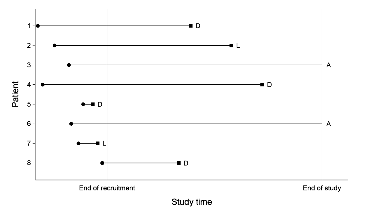
The chronological time needed to observe the lifetimes of all individuals in a study may be large enough that practical constraints prevent full observations
If an individual’s lifetime is only known to be exceed a certain value, then it is known as “censored” observation and the process is known as censoring
For example, if a life test is terminated after 28 days and one item had not failed by then, then we would only know that its lifetime is greater than 28 days and it is referred as “censoring time”
There are different types of censoring, e.g. right, left and interval censoring, which will be discussed in detail in the next chapter
Example 1.1.5
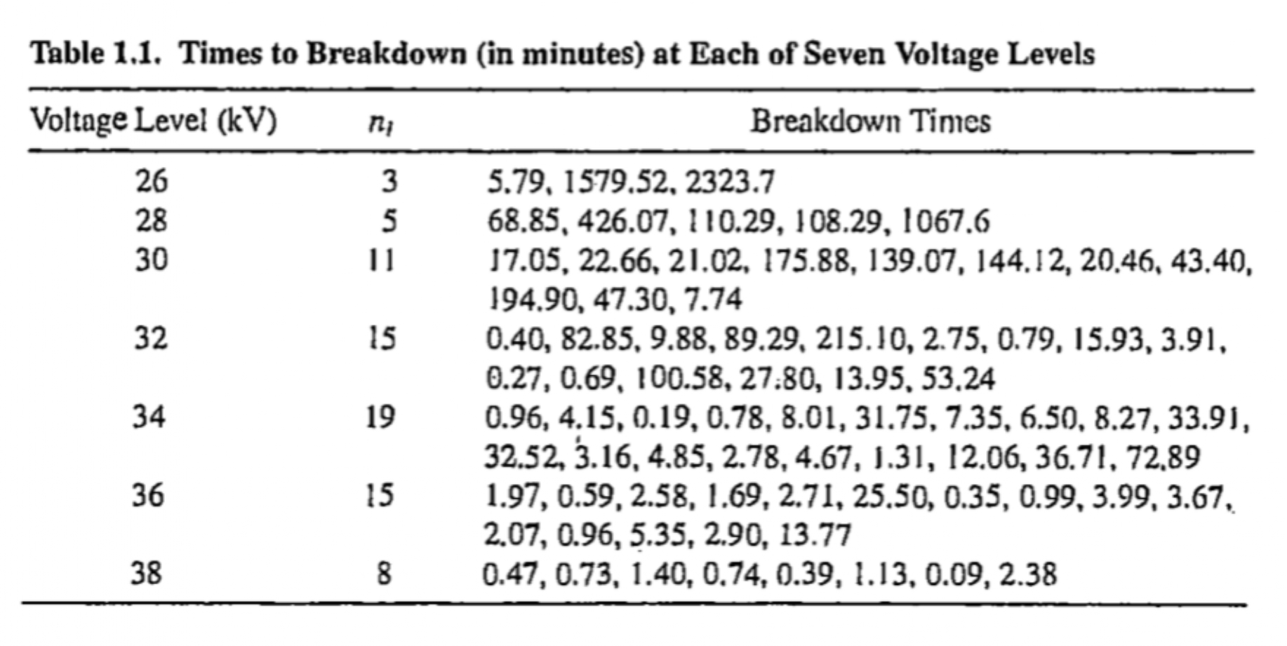
Nelson (1972) described the results of a life test experiment in which specimens of a type of electrical insulating fluid were subjected to a constant voltage stress.
The length of time until each specimen failed, or “broke down,” was observed.
The table in the next slide gives results for seven groups of specimens, tested at voltages ranging from 26 to 38 kilo-volts (kV).
Example 1.1.5
Example 1.1.5
The main purpose of the experiment was to investigate the distribution of “time to breakdown” for the insulating fluid and to relate this to the voltage level
- breakdown times tend to decrease as the voltage increases.
The experiment was run long enough to observe the failure of all the insulation specimens tested.
If a decision had been made in the preceding experiment to terminate testing after 180 minutes had elapsed, then two of the observations in the 26- and 28-kV sample and one each in the 30- and 32-kV samples would have been censored.
- In each case, we would not know the exact failure time of the item, but only that it exceeded 180 minutes.
Example 1.1.7
Gehan (1965) have discussed the results of a clinical trial, in which the drug 6-mercaptopurine (6-MP) was compared to a placebo with respect to the ability to maintain remission in acute leukemia patients.
Remission times for two groups of 21 patients each, one group given the placebo and the other the drug 6-MP are available.

1.2 Lifetime Distributions
Distribution function
Let \(T\) be a nonnegative random variable representing lifetimes of individuals in some population
Let \(f(t)\) be the probability density function (pdf) of \(T\) and the cumulative density function (cdf) of \(T\) can be defined as \[\begin{align} F(t) = \text{Pr}(T\leq t) = \int_0^t f(x) \,dx \end{align}\]
Survivor function
The probability that an individual survives to time \(t\) is given by the survivor function \[\begin{align} S(t) = \text{Pr}(T\geq t) =\int_t^{\infty} f(x)\,dx \end{align}\]
In some context involving lifetimes of manufactured items, \(S(t)\) is referred to as the reliability function
The survivor function \(S(t)\) is a monotone decreasing function with \[S(0)=1\;\; \text{and}\;\; S(\infty)=\lim_{t\to \infty} S(t) =0.\]
A useful relationship \[\begin{align} E(T) = \int_0^\infty S(x)\, dx \end{align}\]
- The mean survival time is the area under the survivor curve
Quantiles
The \(p^{\text{th}}\) quantile of the distribution of \(T\) is the value \(t_p\) such that \[\text{Pr}(T\leq t_p) =F(t_p) = p\;\;\;{\color{red}\Rightarrow}\;\;\;t_p = F^{-1}(p)=S^{-1}(1-p)\]
The \(p^{\text{th}}\) quantile \(t_p\) is also known as \(100p^{\text{th}}\) percentile.
The 0.5 quantile \(t_{.5}\) is called the median of the distribution.
Mortality rate
In life table, the mortality rate at time \(t\) is the proportion of population who die between times \(t\) and \((t + 1)\) among individuals alive at time \(t\) \[\begin{align} q_{\mathrm{t}} = \text{Pr}\big(t \leq T < t + 1 \,\vert\, T \geq t\big) \end{align}\]
- Mortality rate is probability and it lies between 0 and 1
Calculating the mortality rate for ever smaller intervals of time results in the hazard function (also called hazard rate), \(h(t)\).
Hazard function
Hazard function \(h(t)\) is an important concept for lifetime distributions and it can be defined as the limit of the mortality rate \[\begin{align} h(t) &= \lim_{\Delta t\rightarrow 0} \frac{\text{Pr}(t\leq T<t+\Delta t\mid T\geq t)}{\Delta t}\notag\\[.25em] %&= \lim_{\Delta t\rightarrow 0} \frac{\text{Pr}(t\leq T<t+\Delta t, T\geq t)}{\Delta t\;\text{Pt}(T\geq t)}\\ %&=\lim_{\Delta t\rightarrow 0} \frac{\text{Pr}(t\leq T<t+\Delta t)}{\Delta t\;\text{Pt}(T\geq t)}\\ &=\frac{f(t)}{S(t)} \end{align}\]
Hazard function \(h(t)\) specifies instantaneous rate of failure at time \(t\) given that the individual survives up to time \(t\).
Hazard function is conditional failure rate not probability (so can take any positive value, i.e. between 0 to \(\infty\), unlike the mortality rate which is bounded by one)
For a mortality rate \[P = \text{Pr}(t\leq T<t + \Delta t\,\vert\, T\geq t) = 1/4,\] the corresponding hazard rate depends on the length of the interval \(\Delta t\)
The probability that an individual fails in \([t, t+\Delta t)\) given that the individual survives up to time \(t\) is approximated by \[\begin{align} h(t)\Delta t \approx \text{Pr}(t\leq T<t+\Delta t\mid T\geq t) \end{align}\]
The \(h(t)\) can also be regarded as the expected number of events experienced by an individual in unit time, given that the event has not occurred before then, and assuming that the hazard is constant over that time period.
Hazard functions are sometimes given other names, such as conditional failure rate, hazard rate, force of mortality, etc.
Relationship between different functions
The functions \(f(t)\), \(F(t)\), \(S(t)\), and \(h(t)\) give mathematically equivalent specifications of the distribution of \(T\)
From a given expression of one function, say hazard function, expressions of other functions (e.g. density function) can be derived
Expressing \(S(t)\) in terms of \(h(t)\)
. . .
\[ \begin{aligned} h(x) &= \frac{f(x)}{S(x)} = -\frac{d}{dx}\log S(x) \end{aligned} \]
. . .
\[ \begin{aligned} \int_0^t h(x) \,dx & = \int_0^t \Big[ -\frac{d}{dx}\log S(x) \Big]dx \end{aligned} \]
. . .
\[ \begin{aligned} -\int_0^t h(x) \,dx & = \log S(x) \bigg\vert_0^t \\ -\int_0^t h(x) \,dx & = \log S(t) - \log S(0) \end{aligned} \]
. . .
Note \(S(\infty) = 0\) and \(S(0)=1\)
Expressing \(S(t)\) in terms of \(h(t)\)
\[ -\int_0^t h(x) \,dx = \log S(t) \;\;{\color{red}\Rightarrow}\;\; S(t) = \exp\Big(-\int_0^t h(x) \,dx \Big) \]
It is useful to define the cumulative hazard function as \[\begin{align} H(t) = \int_0^t h(x)\,dx \end{align}\]
Cumulative hazard function
Relationship between \(S(t)\) and \(H(t)\) \[ S(t) = \exp\Big(-H(t)\Big) \;\;{\color{red} \Rightarrow}\;\; H(t) = -\log S(t) \]
- \(S(\infty)=0\;\;\Rightarrow\;\;H(\infty) = \infty\)
For a given time \(t\), the greater the risk, the smaller \(S(t)\), and hence the shorter mean survival time \(E(T)\), and vice verse
It is possible for the cumulative hazard function to exceed unity \[ \begin{aligned} H(t) \geq 1 \;\Rightarrow\; -\log\,S(t) \geq 1 \;\Rightarrow\; S(t) \leq e^{-1} = 0.368 \end{aligned} \]
The cumulative hazard is then greater than unity when the probability of an event occurring after time \(t\) is less than 0.37
Relationship between different functions
Expressing \(f(t)\) in terms of \(h(t)\)
\[ \begin{aligned} h(t) & = \frac{f(t)}{S(t)} \\[.25em] f(t) & = h(t) S(t) = h(t)\, \exp\Big(-\int_0^t h(x) \,dx \Big) \end{aligned} \]
Example 1.2.1
Suppose \(T\) has p.d.f. \[ f(t) = \beta t^{\beta-1} \exp(-t^\beta), \; t > 0 \]
- Obtain survivor function and hazard function of \(T\)
Some remarks on hazard functions
The hazard function is an important characteristic of a lifetime distribution that indicates the way the risk of failure varies with age or time, and this is of interest in most applications.
In many instances, information is available on how failure rates change with time and such prior information about the shape of the hazard function can help guide model selection.
The model/information for hazard function can easily be translated for survivor and density functions using the formulas derived earlier
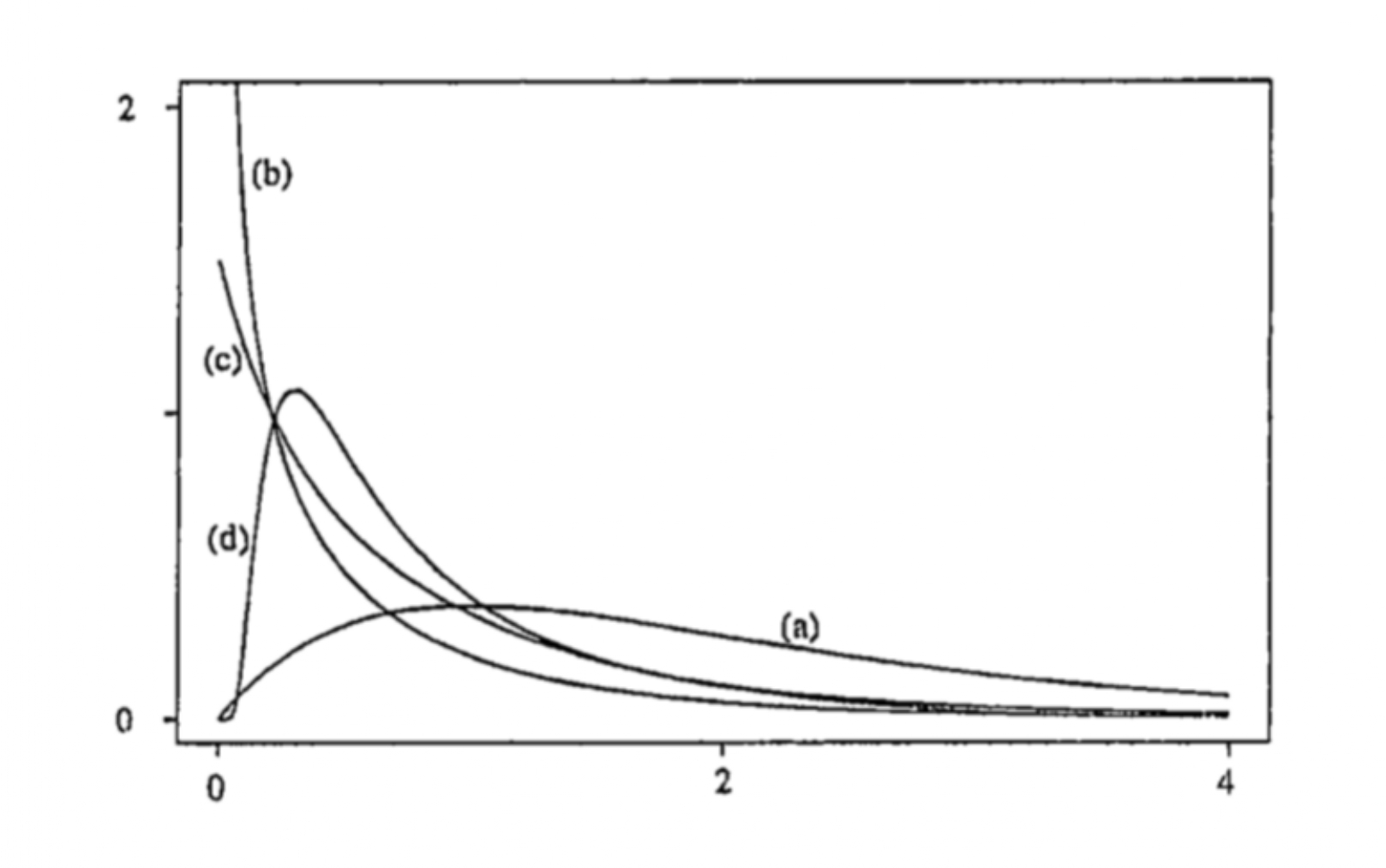
Different shapes of hazard functions
The shapes of hazard functions could be different, such as
monotone increasing (e.g. positive aging)
(a)monotone decreasing (e.g. negative aging)
(b)bathtub-shaped or U-shaped (e.g. age at death of human populations, lifetime of manufactured items, etc.)
(c)inverse bathtub-shaped (e.g. survival after treatment for cancer, duration of marriage, etc.)
(d)
Different shapes of hazard functions
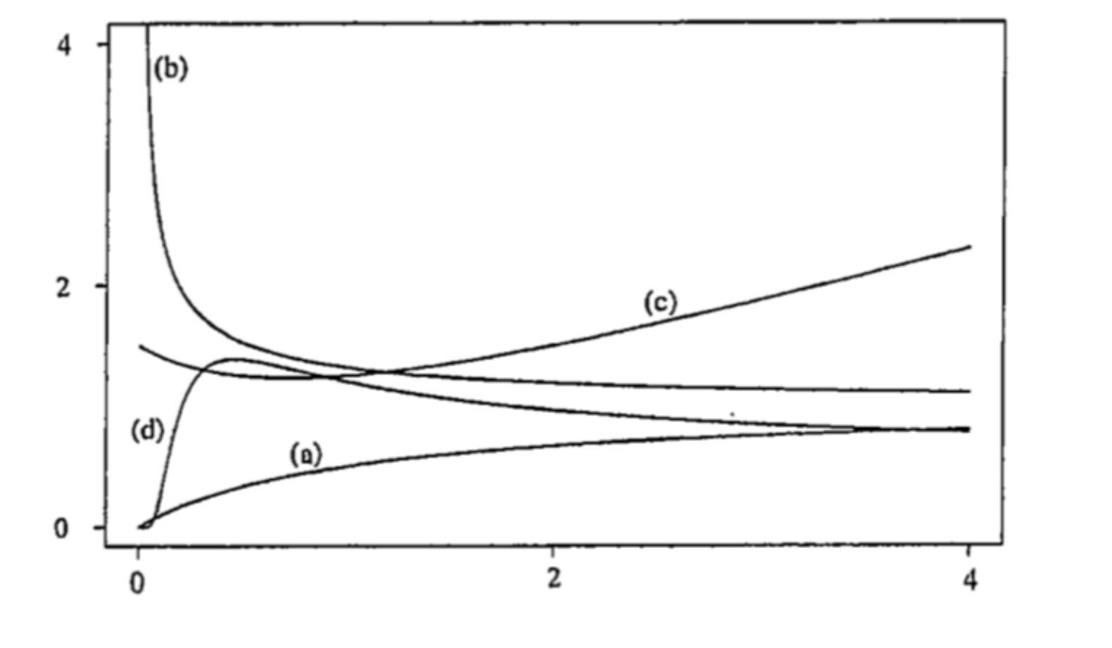
Different shapes of density functions
Some remarks on hazard functions
Shapes of density function could be different corresponding to the shapes of hazard functions
Although different survivor functions can have the same basic shape, their hazard functions can differ dramatically
The hazard function is usually more informative about the underlying mechanism of failure than the survivor function.
Modelling the hazard function is an important method for summarizing survival data
1.3 Some important failure time models
Introduction
Various parametric families of models are used in the analysis of lifetime data and a few distributions have the usefulness in a wide-range of situations
The most commonly used univariate distributions for failure time data
- exponential, Weibull, log-normal, and log-logistic
Notations
\(T\,\rightarrow\) lifetime, takes only nonnegative values, i.e. from 0 to \(\infty\)
\(Y = \log T\,\rightarrow\) log-lifetime, takes any value on the real line, i.e. from \(-\infty\) to \(\infty\)
The exponential distribution
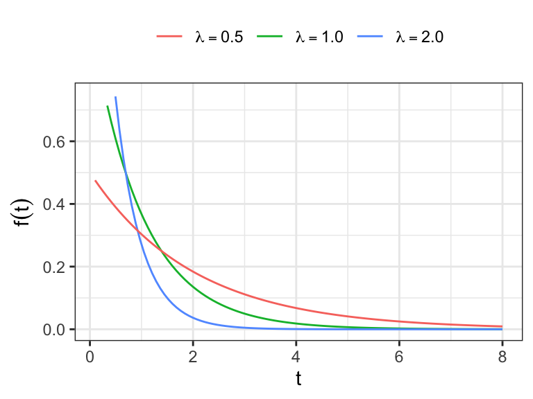
The exponential distribution is characterized by a constant hazard function \[h(t) = \lambda, \;t\geq 0 \]
- \(\lambda >0\)
The cumulative hazard function \[ H(t) = \int_0^t h(x)\,dx = \int_0^t \lambda\,dx = \lambda t \]
The survivor function \[ \begin{aligned} S(t) &= \exp(- H(t)) \\[.25em] & = \exp(-\lambda t) \end{aligned} \]
The probability distribution function \[ \begin{aligned} f(t) & = {\color{red} h(t)}\,{\color{blue} S(t)} = {\color{red}\lambda}\,{\color{blue}\exp(-\lambda t)} \end{aligned} \]
Reprametrization \(\theta = \lambda^{-1}\) Then, \(T\sim \text{Exp}(\text{scale}=\theta)\), where
\[ f(t) = (1/\theta)\,\exp(-t/\theta), \;\;t\geq 0 \]
Properties
\(E(T) = \theta\)
\(V(T) = \theta^2\)
Quantiles, the \(pth\) quantile \[ \begin{aligned} F(t_p) = p & \;\Rightarrow \;1 - \exp(-t/\theta) = p \; \\ & \; \Rightarrow {\color{purple} t_p = -\theta \log(1-p)} \end{aligned} \]
- The median, \(.5th\) quantile \[ t_{.5} = -\theta\log(.5) \]
The exponential distribution with \(\theta = 1\) is known as standard exponential distribution
If \(T\sim \text{Exp}(\theta)\) then \[ (T/\theta)\sim \text{Exp}(1) \]
The mean and variance of \(\text{Exp}(1)\) is 1
The median of the \(\text{Exp}(1)\) is \(-\log(.5)=0.6931\)
The density function of \(\text{Exp}(1)\) is positively skewed
Historically, the exponential was the first widely discussed lifetime distribution model
- This was in part because of the availability of simple statistical methods for it
The assumption of a constant hazard function is very restrictive, so the model’s applicability is fairly limited
The Weibull distribution
The Weibull distribution is the most widely used lifetime distribution model.
It has applications to the lifetimes or durability of manufactured
- It is used as a model with diverse types of items, such as ball bearings, automobile components, and electrical insulation.
It is also used in biological and medical applications, for example, in studies on the time to the occurrence of tumors in human populations or in laboratory animals.
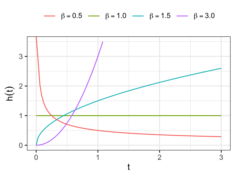
The hazard function of Weibull distribution \[ h(t)=\lambda\beta(\lambda t)^{\beta-1},\;\lambda>0,\;\beta>0. \]
Show that \(h(t)\) is
monotone increasing for \(\beta>1\)
monotone deccreasing for \(\beta<1\)
constant for \(\beta=1\)
Exponential distribution is a special case
- For \(\beta=1\), Weibull distribution reduces to exponential distribution with \(h(t)=\lambda\)

The cumulative hazard function \[ H(t)=\int_0^t \,h(x)\,dx= \int_0^t \lambda\beta\, (\lambda x)^{\beta-1}\,dx=(\lambda\,t)^{\beta} \]
The survivor function \[ S(t) = \exp[-H(t)] = \exp[-(\lambda t)^\beta] \]
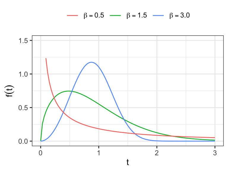
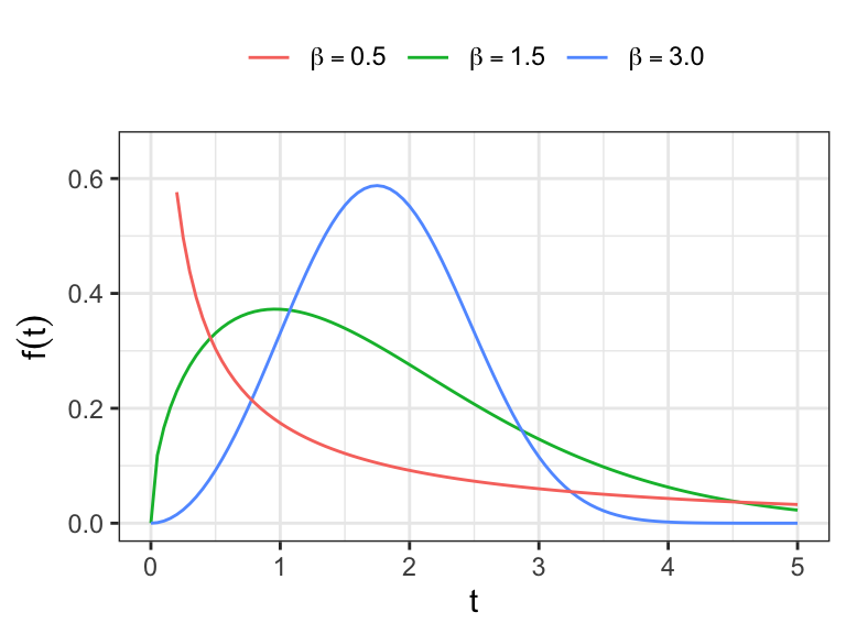
The density function \[ f(t) = h(t)\, S(t) = \lambda\beta\, (\lambda t)^{\beta-1}\exp[-(\lambda t)^\beta] \]
Show that the \(rth\) moment of Weibull distribution \[E(T^r) = \lambda^{-r}\Gamma{(1 + r/\beta)}\]
- Obtain the expressions of \(E(T)\) and \(V(T)\)
The \(p^{\text{th}}\) quantile can be obtained as \[F(t) = 1-e^{-(\lambda t_p)^{\beta}}=p \;\;\Rightarrow\;\; t_p=\alpha[-\log(1-p)]^{1/\beta}\]
\(\alpha = 1/\lambda\) is known as the scale parameter of the distribution
The shape of the distribution depends on \(\beta\), which is known as the shape parameter
It can be shown that \(\alpha\) is the .632 quantile of the distribution irrespective of the value of \(\beta\)
- i.e. \(\alpha\) is greater than the median of the distribution!
The extreme value distribution
Let \(T\) follows a Weibull distribution \[ T\sim \text{Weib}(\alpha, \beta)\;\;\text{with}\;\; \alpha = 1/\lambda \]
Extreme value distribution (also known as Gumbel distribution) is closely related to Weibull distribution
If lifetime \(T\) follows a Weibull distribution then log-lifetime \(Y = \log T\) follows an extreme value distribution
Extreme value distribution has two parameters, which have one-to-one connection with the Weibull distribution parameters!
\(T \sim \text{Weib}(\alpha, \beta)\;\;\Leftrightarrow\;\;Y = \log T\sim \text{EV}(u, b)\)
\(u = \log\alpha\) and
\(b = (1/\beta)\)
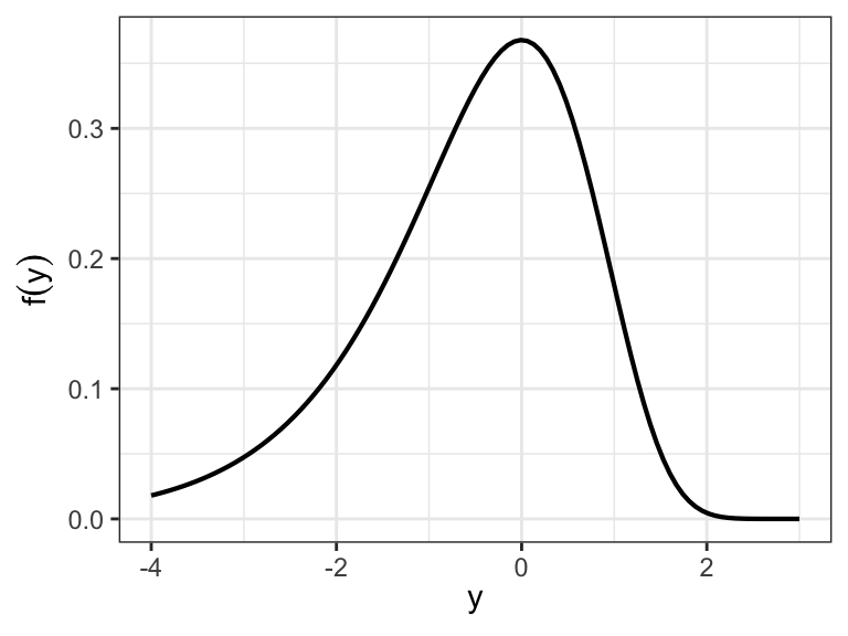
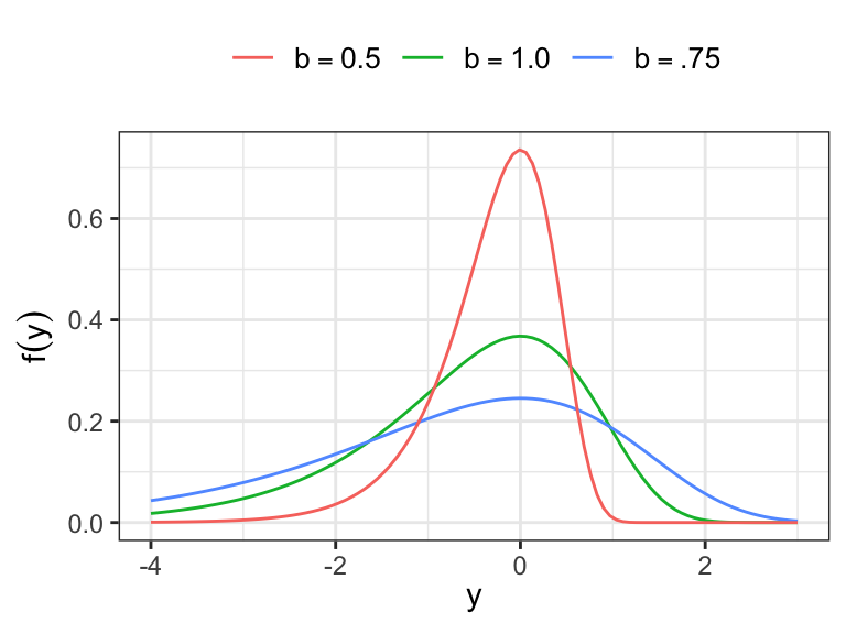
The pdf of \(Y\) \[ f(y) = (1/b)\exp\Big[\frac{y-u}{b}-\exp\Big(\frac{y-u}{b}\Big) \Big]\;\;-\infty< y <\infty \]
- \(-\infty < u < \infty\) and \(b>0\)
Exercise: obtain the pdf of \(Y=\log T\), where \(T\sim \text{Weib}(\alpha, \beta)\)
- Hints. \(J = \frac{dt}{dy} = e^y\) and \[ f_Y(y) = f_T(e^y)\;\vert\, J\,\vert \]
The survivor function \[ \begin{aligned} S(y) &= \int_y^{\infty} f(x\,dx) \\ & = \int_y^{-\infty} (1/b)\exp\Big[\frac{x-u}{b}-\exp\Big(\frac{x-u}{b}\Big) \Big]\,dx \\ & = \exp\Big[-\exp\Big(\frac{y - u}{b}\Big)\Big] \end{aligned} \]
The cumulative hazard function \[ H(y) = \exp\Big(\frac{y-u}{b}\Big) \]
The hazard function \[ h(y) = \frac{d\,H(y)}{dy} = (1/b)\exp\Big(\frac{y-u}{b}\Big) \]
Standard extreme value distribution
- If \(Y\sim \text{EV}(u, b)\), then \[ \frac{Y-u}{b} \sim \text{EV}(0, 1), \] the standard extreme value distribution.
- The moment generating function of \(EV(u, b)\) \[
\begin{aligned}
M(\theta) &= \int_{-\infty}^\infty e^{\theta y} \,f(y)\, dy\\[.25em]
& = \int_{-\infty}^\infty e^{\theta y}\,(1/b)\,\exp\Big[\frac{y-u}{b} - \exp\Big(\frac{y-u}{b}\Big)\Big]dy
\end{aligned}
\]
- Let \((y-u)/b = z\) \[ \begin{aligned} M(\theta) &= \int_{-\infty}^\infty e^{\theta(u + bz)}\exp\big[z - \exp(z)\big]dz \end{aligned} \]
- Let \(e^z =x\) \[ M(\theta) = \int_0^\infty e^{\theta u}\, x^{\theta b}\, e^{-x}\, dx = e^{\theta u}\,\Gamma{(\theta b + 1)} \]
If \(Y\sim EV(u, b)\) \[ M(\theta) = e^{\theta u}\, \Gamma(\theta b + 1) \]
If \(Y\sim EV(0, 1)\) \[ M(\theta) = \Gamma(\theta + 1) \]
Moments of standard extreme value distribution \(Z\sim EV(0, 1)\) \[ \begin{aligned} E(Z) &= \frac{d}{d\theta}M(\theta)\big\vert_{\theta=0}=\Gamma'(1)=-\gamma\;\; (\text{Euler's constant})\\[.25em] V(Z) & = \Gamma''(1) - \gamma^2 = \pi^2/6 \end{aligned} \]
For \(Y \sim EV(u, b)\), show that \[ E(Y) =u - \gamma b\;\;\text{and}\;\; V(Y) = b^2(\pi^2/6) \]
The \(pth\) quantile of extreme value distribution
\[ \begin{aligned} F(y_p) & = p \\ S(y_p) &= 1-p \\ %\exp\Big[-\exp\Big(\frac{y_p-u}{b}\Big) \Big] &= (1-p)\\ %\frac{y_p-u}{b} & = \log\big[-\log(1-p)] \\ y_p & = u + b\log\big[-\log(1-p)] \end{aligned} \]
- Show that the location parameter \(u\) is the .632 quantile of \(Y\sim EV(u, b)\)
The log-normal distribution
The lifetime \(T\) is said to be log-normally distributed if log-lifetime \(Y=\log T\) is normally distributed.
The parameters of normal distribution \(\mu\) and \(\sigma\) are also considered as the parameters of log-normal distribution \[Y=\log T \sim N(\mu, \sigma^2)\;\Rightarrow\;T = \exp(Y)\sim \log N(\mu, \sigma^2)\]
- Let \(Y=\log T \sim N(\mu, \sigma^2)\), show that the density function of \(T=\exp(Y)\) \[
\begin{aligned}
f_T(t) &= f_Y(\log T) \bigg\vert \frac{dy}{dt}\bigg\vert \\
& = \frac{1}{\sigma t\sqrt{2\pi}}\exp\Bigg[-\frac{1}{2}\Bigg(\frac{\log t - \mu}{\sigma}\Bigg)^2 \Bigg]
\end{aligned}
\]
- \(t>0\), \(\sigma>0\), and \(-\infty < \mu < \infty\)
The survivor function of \(T=\exp(Y)\) \[ S(t) = 1 - \Phi\bigg(\frac{\log t - \mu}{\sigma}\bigg) \]
- \(\Phi(\cdot)\;\rightarrow\) distribution function of \(N(0, 1)\)
The hazard function is defined as \(f(t)/S(t)\), which takes the value 0 at \(t=0\), increases to a maximum and then decrease, approaching 0 as \(t\to \infty\).
It can be shown \[ \begin{aligned} E(T) &= \exp(\mu + \sigma^2/2)\\[.25em] V(T)&=[\exp(\sigma^2)-1][\exp(2\mu + \sigma^2)] \end{aligned} \]
For log-normal distribution
\(\exp(\mu)\;\rightarrow\) the scale parameter
\(1/\sigma\;\rightarrow\) the shape parameter
Show that for \(T\sim \log N(\mu,\sigma^2)\) \[ t_{.5} = \exp(\mu) \]
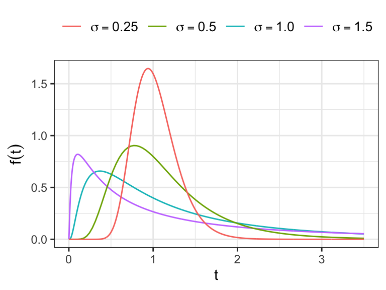
The Log-logistic distribution
If \(Y = \log T\) follows a logistic distribution then \(T\) follows a log-logistic distribution
The p.d.f. of a logistic distribution with parameters \(u\) and \(b\) \[ f(y) = \frac{(1/b)\exp\big[(y-u)/b\big]}{\big\{1 + \exp\big[(y-u)/b\big]\big\}^2} \]
- \(-\infty < y <\infty\), \(-\infty < u < \infty\), \(b>0\)
The survivor function of a logistic distribution \[ S(y) = \frac{1}{\big\{1 + \exp\big[(y-u)/b\big]\big\}} \]
The hazard function of logistic distribution \[ h(y) = \frac{(1/b) \exp\big[(y-u)/b\big]}{\big\{1 + \exp\big[(y-u)/b\big]\}} \]
The p.d.f. of log-logistic distribution \[ \begin{aligned} f_T(t) &= f_Y(\log T)\,\Big\vert \frac{dy}{dt}\Big\vert\\[.25em] & = \frac{(\beta/\alpha)(t/\alpha)^{\beta-1}}{\big[1+ (t/\alpha)^\beta\big]^2} \end{aligned} \]
- \(\alpha = \exp(u) > 0\) and \(\beta = 1/b > 0\)
The survivor function of \(T\sim \text{LLogis}(\alpha, \beta)\) \[ \begin{aligned} S(t) &= \int_t^\infty \frac{(\beta/\alpha)(x/\alpha)^{\beta-1}}{\big[1+ (x/\alpha)^\beta\big]^2}\, dx \end{aligned} \]
- Let \((x/\alpha)^\beta=y\) \[ \begin{aligned} S(t) &= \int_{(t/\alpha)^\beta}^\infty \frac{1}{(1+ y)^2}\, dy\\[.25em] & = \frac{-1}{1+ y}\Bigg\vert_{(t/\alpha)^\beta}^\infty\\[.25em] & = \big[1+ (t/\alpha)^\beta \big]^{-1} \end{aligned} \]
The p.d.f. \[ f(t) = \frac{(\beta/\alpha)(t/\alpha)^{\beta-1}}{\big[1+ (t/\alpha)^\beta\big]^2} \]
The survivor function \[ S(t) = \big[1+ (t/\alpha)^\beta \big]^{-1} \]
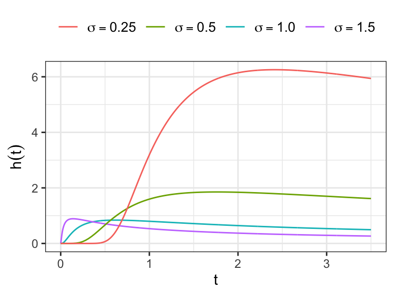
The hazard function \[ h(t)= \frac{(\beta/\alpha)(t/\alpha)^{\beta-1}}{\big[1+ (t/\alpha)^\beta\big]} \]
- Show that for \(T\sim \text{LLogis}(\alpha, \beta)\), provided \(\beta>r\) \[ E(T^r) = \alpha^r\,\Gamma(r/\beta +1)\Gamma(1-r/\beta) \]
- Beta distribution of the first kind \[ f(x; \alpha, \beta) = \frac{1}{\text{Beta}(\alpha, \beta)}\, x^{\alpha-1}\,(1-x)^{\beta-1}\;\;\;\;\;\;0< x < 1 \]
- Beta distribution of the second kind \[ f(x; \alpha, \beta) = \frac{1}{\text{Beta}(\alpha, \beta)}\,\frac{x^{\alpha-1}}{(1 + x)^{\alpha + \beta}}\;\;\;\;\;\;x > 0 \]
The logistic and normal distribution have similar shapes
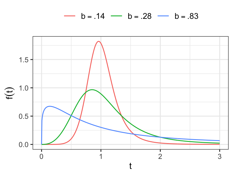
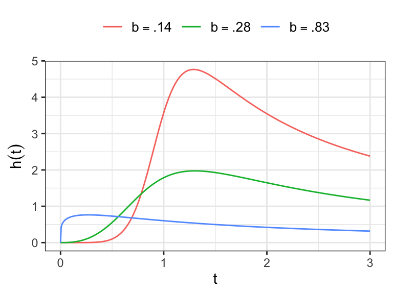
For \(\beta>1\), the hazard function of log-logistic distribution has the same characteristic as that of log-normal distribution, i.e. \(h(0)=0\), increases to maximum and then approaches 0 monotonically as \(t\to \infty\).
For \(\beta<1\), the hazard function is monotone decreasing
The gamma distribution
- The gamma distribution has a pdf of the form \[
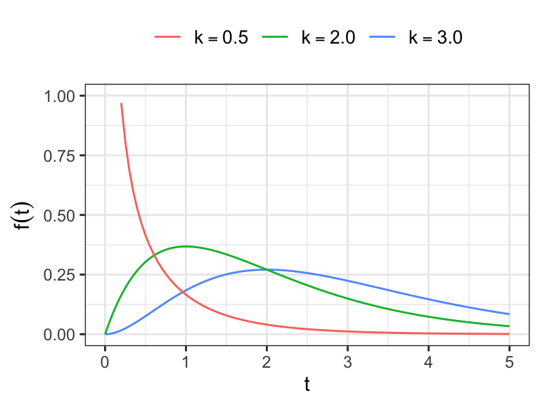
f(t) = \frac{\lambda(\lambda t)^{k-1}\,e^{-\lambda t}}{\Gamma(k)}\;\;\;t>0
\]
\(k>0\) and \(\lambda >0\)
\(\lambda^{-1}\,\rightarrow\) scale parameter
\(k\,\rightarrow\) shape parameter
- For \(k=1\), gamma distribution reduces to exponential distribution
- Incomplete gamma function
\[ I(k, x) = \frac{1}{\Gamma(k)}\int_0^x u^{k-1}\, e^{-u}\, du \]
Survivor function \[ S(t) = \int_t^\infty \frac{\lambda(\lambda x)^{k-1}\,e^{-\lambda x}}{\Gamma(k)}\, dx \]
- Let \(\lambda x = t\) \[ S(t) = \frac{1}{\Gamma(k)}\int_{\lambda t}^\infty y^{k-1}\,e^{-k}\,dy=1-I(k, \lambda t) \]
The hazard function \[ h(t) = \frac{f(t)}{S(t)} \]
For \(k>1\), with \(h(0)=0\) and \(\lim_{t\to 0}\,h(t)=\lambda\)
\(0<k<1\), \(h(t)\) is monotone decreasing, with
\[\lim_{t\to 0}h(t)=\infty\; and \;\lim_{t\to \infty}h(t)=\lambda\]
The distribution with \(\lambda=1\) is called one-parameter gamma distribution, denoted by \(Ga(k)\), and has p.d.f. \[ f(t) = \frac{t^{k-1}\,e^{-t}}{\Gamma(k)}\;\;\;t>0 \]
If \(T\) follows a gamma distribution with scale parameter \(\lambda^{-1}\) and shape parameter \(k\), then show that \(\lambda T\sim Ga(k)\)
- Hints. \(Y=\lambda T\) and \(f_Y(y) = f_T(y/\lambda)\, \vert dt/dy \vert\)
If \(Y\sim Ga(k)\) then \(2Y\sim \chi^2_{(2k)}\)
Let \(T_1, \ldots, T_n\) are independent and identical and exponentially distributed with parameter \(\lambda\)
- \(\sum_{i=1}^n T_i\) follows a gamma distribution with parameters \(\lambda\) and \(n\)
The moment generating function of \(Y\sim Ga(k)\) is \(M(\theta) = (1-\theta)^{-k}\)
Log-Location-scale models
Definition: Location Scale Family A location-scale family is a family of distributions formed by translation and rescaling of a standard family member.
A parametric location-scale model for a random variable \(Y\) is a distribution with p.d.f. of the form \[ f(y) = \frac{1}{b}\,\,f_0\bigg(\frac{y-u}{b}\bigg)\;\;-\infty<y<\infty \]
\(-\infty<u<\infty\), location parameter
\(b>0\), scale parameter
\(f_0(z)\) is a specified p.d.f. on \((-\infty, \infty)\)
The cumulative density function of \(Y\) \[ \begin{aligned} F(y) &= \int_{-\infty}^y (1/b)\, f_0\bigg(\frac{x-u}{b}\bigg)\,dx \\[.25em] & = \int^{(y-u)/b}_{-\infty} f_0(z)\,dz \\[.25em] & = F_0\bigg(\frac{y-u}{b}\bigg) \end{aligned} \]
Similarly, the survivor function of \(Y\) \[ S(y) = 1 - F_0\bigg(\frac{y-u}{b}\bigg) = S_0\bigg(\frac{y-u}{b}\bigg) \]
The distribution of the standardized variable \(Z = (Y-u)/b\)
Probability density function of \(Z\) \[ f_Z(z) = f_Y\bigg(\frac{y-u}{b}\bigg)\,\Big\vert \frac{dy}{dz}\Big\vert = (1/b)\,f_0(z)\,(b) = f_0(z) \]
Survivor function of \(Z\) \[ S_Z(z) = \int_z^\infty f_0(x)\, dx = S_0(z) \]
Cumulative density function of \(Z\) \[ F_Z(z) = F_0(z) \]
- There is an one-to-one correspondence between some lifetime and log-lifetime distributions
Parameters of lifetime distributions \[\text{scale ($\alpha$) and shape ($\beta$)}\]
Parameters of log-lifetime distributions \[\text{location ($u=\log\alpha$) and scale ($b = 1/\beta$)}\]
For the standardized log-lifetimes \(Z=(Y-u)/b\)
The density, cumulative density, and survivor functions can be expressed in terms of \(f_0(\cdot)\), \(F_0(\cdot)\), and \(S_0(\cdot)\), respectively
For example, the survivor functions of log-lifetimes are defined as \[ \begin{aligned} S_0(z) &= \exp(-e^z) \;\longrightarrow\;\text{extreme value}\\[.25em] S_0(z) &= 1- \Phi(z) \;\longrightarrow\;\text{normal}\\[.25em] S_0(z) &= (1 + e^z)^{-1} \;\longrightarrow\;\text{logistic} \end{aligned} \]
Using the transformation \(T=\exp(Y)\), lifetime distributions can be obtained from each of the distributions of location-scale family \[ \begin{aligned} S_T(t) &= P(T\geq t)\\[.25em] & = P(\log T \geq \log t) \\[.25em] %& = P\bigg(\frac{Y - u}{b} \geq \frac{\log t - u }{b}\bigg) \\[.25em] & = S_0\bigg(\frac{\log t -u}{b} \bigg) \\[.25em] %& = S_0\bigg(\log\Big(\frac{t}{\alpha}\Big)^\beta\bigg)\\[.25em] & = S_0^\star\bigg(\Big(\frac{t}{\alpha}\Big)^\beta\bigg) \end{aligned} \]
- \(S_0^\star(x) = S_0(\log x)\)
Obtain the survivor function of \(T\sim \text{Weib}(\alpha, \beta)\) from \(Y\sim EV(u, b)\) \[ \begin{aligned} S(t) & = S_0^\star\Big(\big({t}/{\alpha}\big)^\beta\Big) \\[.25em] & = S_0\Big(\log \big({t}/{\alpha}\big)^\beta\Big)\\[.25em] & = \exp\Big(-e^{\log\big(t/\alpha\big)^\beta}\Big)\\[.25em] & = \exp\Big(-{\big(t/\alpha\big)^\beta}\Big) \end{aligned} \]
Similarly, obtain the expressions of survivor function of log-logistic and log-normal distribution using the relationship \(S(\cdot)=S_0^\star(\cdot)\)
1.4 Regression models
Regression models
Regression models are used to understand the relationship between lifetime and a set of covariates (e.g. age, gender, disease status, values of bio-markers, etc.), some of which may depend on time
Regression models considered for lifetimes can be divided into two broad categories
parametric models
semiparametric models
Parametric regression models
Parametric models discussed in this chapter (e.g. Weibull, log-logistic, etc.) can be considered for modeling lifetime
In parametric regression model, one of the parameters of the assumed lifetime distribution is expressed as a function of available covariates
Let \(T\) be the lifetime and \(\mathbf{x}=(x_1, \ldots, x_p)'\) be the available \(p\) covariates
Assume \(T\sim \text{Exp}(\theta)\) and since \(\theta>0\), a reasonable model for \(\theta\) would be \[\theta(\mathbf{x}) = \exp\big(\boldsymbol{\beta}'\mathbf{x}\big), \;where\; \boldsymbol{\beta} = (\beta_1, \ldots, \beta_p)'\]
The model specification \(\theta(\mathbf{x}) = \exp\big(\boldsymbol{\beta}'\mathbf{x}\big)\) ensures \(\theta(\mathbf{x}) \geq 0\) for any set of values of \(\boldsymbol{\beta}\) and \(\mathbf{x}\)
For the given set of covariates \(\mathbf{x}\), the survivor function is defined as \[ S(t\,\vert\, \mathbf{x}) = \exp(-t/\theta(\mathbf{x})) \]
If \(Y=\log T\) follows a distribution of location-scale family, the model \(u(\mathbf{x}) = \boldsymbol{\beta}'\mathbf{x}\) would be useful, \(-\infty <u(\mathbf{x})<\infty\)
The corresponding survivor function has the form \[ S_Y(y\,\vert\, \mathbf{x}) = P(Y\geq y\,\vert\,\mathbf{x}) = S_0\bigg(\frac{y-u(\mathbf{x})}{b}\bigg) \]
- For example, if \(S_0(\cdot)\) is the survivor function of standard normal distribution, then the model \(u(\mathbf{x}) = \boldsymbol{\beta}'\mathbf{x}\) represents the multiple linear regression model!
Semiparametric regression models
In semiparametric regression model, the dependence of \(Y\) or \(T\) on \(\mathbf{x}\) is specified by a parametric function without making any distributional assumption regarding \(Y\) or \(T\)
For lifetime data, the most famous semiparametric regression mode is Cox’s proportional hazards model (Cox 1972)
Cox’s model cosiders the hazard function of \(T\) given \(\mathbf{x}\) of the form \[ h(t\,\vert\, \mathbf{x}) = h_0(t)\,\exp(\boldsymbol{\beta}'\mathbf{x}) \]
\(h_0(t)\,\longrightarrow\) arbitrary “baseline” hazard function
Time-dependent covariates can be included in Cox’s proportional hazards model
Exercises
- Obtain graphs of probability density, survivor, and cumulative hazard functions of the following distributions using R codes.
Weibull distribution with (i) scale parameter 10, and shape parameter 1.5 and (ii) scale parameter 10, and shape parameter 0.95
Logistic distribution with (i) location parameter 10 and scale parameter 1.5 and (ii) location parameter 10 and scale parameter 0.75
Acknowledgements
This lecture is adapted from materials created by Mahbub Latif