Chapter 2

(AST405) Lifetime data analysis

Author

Affiliation

Md Rasel Biswas

ISRT, University of Dhaka

2 Observed Schemes, Censoring, and Likelihood

2.1 Introduction

Preliminary discussion of likelihood;

• Suppose that the probability distribution of potentially observable data in a study specified up to the parameter vector $\mathit{\theta }$

• A likelihood function for $\mathit{\theta }$ is a function of $\mathit{\theta }$ and is proportional to the probability of data that were observed $$L(\mathit{\theta })\propto Pr(\text{Data};\mathit{\theta })\text{(2.1.1)}$$

  • Data $\to$ observed data

  • $Pr\to$ probability density or mass function from which the data are assumed to arise

  • $L(\mathit{\theta };\text{Data})\to$ is a more formal notation for likelihood function

Asymptotic results and large sample methods

• Assume that the data consist of a random sample $y_1,\dots ,y_n$ from a distribution with probability density function $f(y;\mathit{\theta })$

• $\mathit{\theta }=({\theta }_1,\dots ,{\theta }_k{)}^{\prime }\to$ a vector of unknown parameters, $\mathit{\theta }\in \mathrm{\Omega }$

• $y_i$’s can be vectors, but for simplicity, they are considered scalars

• The likelihood function for $\mathit{\theta }$ $$L(\mathit{\theta })=\prod _{i=1}^{n}f(y_i;\mathit{\theta })$$

• If $y_i$’s are independent but not identically distributed then $f(y_i;\mathit{\theta })$ is replaced by $f_i(y_i;\mathit{\theta })$ in the definition of likelihood function

---

• Let $\hat{\mathit{\theta }}$ be a point in $\mathrm{\Omega }$ at which $L(\mathit{\theta })$ is maximized

  • $\hat{\mathit{\theta }}\to$ maximum likelihood estimator (m.l.e.) of $\mathit{\theta }$

  • In most simple settings $\hat{\mathit{\theta }}$ exists and unique

• It is often convenient to work with the log-likelihood function, which is also maximized at $\hat{\mathit{\theta }}$ $$\begin{array}{r}\ell (\mathit{\theta })=\log L(\mathit{\theta })=\sum _i\log f(y_i;\mathit{\theta })\end{array}$$

---

• The m.l.e. $\hat{\mathit{\theta }}$ can be found by solving $$U_j(\mathit{\theta })=\mathbf{0}(j=1,\dots ,k)$$

  • $U_j(\mathit{\theta })=\frac{\partial \ell (\mathit{\theta })}{\partial {\theta }_j}\to$ $jth$ score or score function

  • $\mathbf{U}(\mathit{\theta })=[U_1(\mathit{\theta }),\dots ,U_k(\mathit{\theta }){]}^{\prime }\to$ score vector of order $k\times 1$

---

• Score vector $U(\mathit{\theta })$ is asymptotically ($k$-variate) normally distributed with mean $\mathbf{0}$ and variance-covariance matrix $\mathcal{I}(\mathit{\theta })$ with the $(j,j^{\prime })th$ entry of $\mathcal{I}(\mathit{\theta })$ $${\mathcal{I}}_{j{j}^{\prime }}(\mathit{\theta })=E(\frac{-{\partial }^2\ell (\mathit{\theta })}{\partial {\mathit{\theta }}_j\partial {\mathit{\theta }}_{j^{\prime }}})j,j^{\prime }=1,\dots ,k$$

  • $\mathcal{I}(\mathit{\theta })\to$ Fisher or expected information matrix

  • $I(\hat{\mathit{\theta }})\to$ observed information matrix

• Under mild regularity conditions

  • $\hat{\mathit{\theta }}$ is a consistent estimator of $\mathit{\theta }$

  • $I(\hat{\mathit{\theta }})/n$ is a consistent estimator of $\mathcal{I}(\mathit{\theta })/n$

Optimization methods for maximum likelihood

• Maximum likelihood estimator $\hat{\mathit{\theta }}$ correspond to the maximum of the log-likelihood function $\ell (\mathit{\theta })$, i.e. $$\begin{array}{r}\hat{\mathit{\theta }}=\arg \underset{\theta \in \mathrm{\Omega }}{max}\ell (\mathit{\theta })\end{array}$$

---

• There are different numerical approaches for optimizing the multiparameter log-likelihood function $\ell (\mathit{\theta })$ for $\mathit{\theta }\in \mathrm{\Omega }$

• Many likelihood functions have a unique maximum at $\hat{\mathit{\theta }}$, which is a stationary point satisfying $\partial \ell (\mathit{\theta })/\partial \mathit{\theta }=\mathbf{0}$

• Numerical approaches involve a starting point ${\mathit{\theta }}_0$ and an iterative procedure designed to give a sequence of points ${\mathit{\theta }}_1,{\mathit{\theta }}_2,\dots$ converging to $\hat{\mathit{\theta }}$ (i.e. when ${\mathit{\theta }}_j\simeq {\mathit{\theta }}_{j-1}$)

---

• Three types of optimization methods are available in statistical software

  • Methods that do not use derivatives (e.g., simplex algorithm, such as Nelder-Mead method)

  • Methods that use only first derivates $U(\mathit{\theta })=\partial \ell (\mathit{\theta })/\partial \mathit{\theta }$ (e.g. steepest ascent, quasi-Newton, and conjugate gradient method)

  • Methods that use both first derivative $U(\mathit{\theta })$ and second derivative $H(\mathit{\theta })={\partial }^2\ell (\mathit{\theta })/\partial \mathit{\theta }\partial {\mathit{\theta }}^{\prime }$ (e.g. Newton-Raphson method)

    • $H(\mathit{\theta })$ is known as Hessian matrix and observed information matrix $I(\hat{\mathit{\theta }})=-H(\hat{\mathit{\theta }})$

---

• Newton-Raphson method is commonly used for optimizing $\ell (\mathit{\theta })$, which is based on the iteration scheme for the $jth$ step $(j=1,2,\dots )$ as $${\mathit{\theta }}_j={\mathit{\theta }}_{j-1}-[H({\mathit{\theta }}_{j-1}){]}^{-1}U({\mathit{\theta }}_{j-1})$$

  • ${\mathit{\theta }}_{j-1}\to$ value of $\mathit{\theta }$ at the $(j-1)th$ iteration

• Using Taylor series expansion, expanding $U(\mathit{\theta })$ at ${\mathit{\theta }}_j$ $$\begin{array}{rl}U(\mathit{\theta })& =U({\mathit{\theta }}_j)+H({\mathit{\theta }}_j)(\mathit{\theta }-{\mathit{\theta }}_j)\end{array}$$
  • Then $$U(\mathit{\theta })=\mathbf{0}\Rightarrow \mathit{\theta }={\mathit{\theta }}_j-[H({\mathit{\theta }}_j){]}^{-1}U({\mathit{\theta }}_j)$$

---

• In many situations, finding the maximum likelihood estimator may be challenging, e.g. it may be on the boundary of $\mathrm{\Omega }$

• Likelihood function may also possess multiple stationary points, and optimization techniques are designed to obtain local maxima, so it may not converge to global maxima

• It is important to understand the shape of $\ell (\mathit{\theta })$ before applying an optimization method

Example 2.1.1

• Suppose that the lifetimes of individuals in some population follow a distribution with density function $f(t)$ and distribution function $F(t)$, and that the lifetimes $t_1,\dots ,t_n$ for a random sample of $n$ individuals are observed.

• In format of Eq. 2.1.1, Data = $(t_1,\dots ,t_n)$ and $$Pr(Data)=\prod _{i=1}^{n}f(t_i)\text{(2.1.2)}$$

Parametric approach

• Assume that $f(t)$ has a specific parametric form $f(t;\mathit{\theta })$

• Likelihood function $$L(\mathit{\theta })=\prod _{i=1}^{n}f(t_i;\mathit{\theta })$$

• The maximum likelihood estimator $\hat{\mathit{\theta }}$ can be obtained by maximizing $L(\mathit{\theta })$ or $\ell (\mathit{\theta })$ and consequently an estimate of $F(t;\hat{\mathit{\theta }})$, the distribution function

• For example, if $T\sim \text{Exp}(\theta )$ then $\hat{\theta }=\overline{t}$ and $F(t;\hat{\theta })=\exp (-t/\hat{\theta })$

Nonparametric approach

• Assume $F(t)$ is discrete with unspecified probabilities $f(t)=F(t)-F(t-1)$ at the jump points $t=1,2,\dots$

• The model parameters are $\mathbf{f}=(f(1),f(2),\dots )$ and the likelihood function is $$L=\prod _{i=1}^{n}f(i)$$

  • Restrictions: $f(t)\ge 0\mathrm{\forall }t\text{and}\sum _{s=1}^{n}f(s)=1$

---

• The maximum likelihood estimators can be obtained by maximizing the corresponding likelihood function $$\hat{f}(t)=\frac{1}{n}\sum _{i=1}^{n}I(t_i=t)$$

  • $I(A)$ is an indicator function $$I(A)=\{\begin{array}{ll}1& \text{if }A\text{ is true}\\ 0& \text{otherwise}\end{array}$$

---

• Estimate of the distribution function $F(t)$ $$\begin{array}{rl}\hat{F}(t)& =\sum _{t_i\le t}\hat{f}(t_i)\\ & =\frac{1}{n}\sum _{i=1}^{n}I(t_i\le t)\end{array}$$

  • $\hat{F}(t)\to$ empirical distribution funciton

Likelihood for a truncated sample

• Suppose that $t_1,\dots ,t_n$ are not from an unrestricted random sample of individuals, but a random sample of those with lifetimes one year or less

  • No information is available for those whose lifetimes are greater than one year

• The likelihood function for this truncated sample is given by $$\prod _{i=1}^{n}Pr(t_i|T_i\le 1)=\prod _{i=1}^n\frac{f(t_i)}{F(1)}$$ rather than (2.1.2)

Likelihood based inferences

Score test

• Score vector $U(\mathit{\theta })$ asymptotically follows $k$-variate normal distribution with mean vector $\mathbf{0}$ and variance-covariance matrix $\mathcal{I}(\mathit{\theta })$

• Under the null hypothesis $H_0:\mathit{\theta }={\mathit{\theta }}_0$ $$\begin{array}{r}W({\mathit{\theta }}_0)=U({\mathit{\theta }}_0{)}^{\prime }\mathcal{I}({\mathit{\theta }}_0{)}^{-1}U({\mathit{\theta }}_0)\end{array}$$ asymptotically follows ${\chi }_{(k)}^2$ distribution.

• The statistic $W({\mathit{\theta }}_0)$ can also be used to obtain confidence intervals for $\mathit{\theta }$

---

Wald test

• The m.l.e. $\hat{\mathit{\theta }}$ follows a $k$-dimensional normal distribution with mean $\mathit{\theta }$ and variance-covariance matrix $\mathcal{I}(\mathit{\theta }{)}^{-1}$

• In other words, $\sqrt{n}(\hat{\mathit{\theta }}-\mathit{\theta })$ follows a $k$-dimensional normal distribution with mean $\mathbf{0}$ and variance-covariance matrix $n\mathcal{I}(\mathit{\theta }{)}^{-1}$

• Under $H_0:\mathit{\theta }={\mathit{\theta }}_0$ $$(\hat{\mathit{\theta }}-{\mathit{\theta }}_0{)}^{\prime }\mathcal{I}({\mathit{\theta }}_0)(\hat{\mathit{\theta }}-{\mathit{\theta }}_0)$$ asymptotically follows ${\chi }_{(k)}^2$.

• Since $I(\hat{\mathit{\theta }})/n$ is a consistent estimator of $\mathcal{I}({\mathit{\theta }}_0)$, we can replace $\mathcal{I}({\mathit{\theta }}_0)$ by $\mathbf{I}(\hat{\mathit{\theta }})$ in the test statistic.

---

Likelihood ratio test

• Under $H_0:\mathit{\theta }={\mathit{\theta }}_0$ $$\begin{array}{rl}\mathrm{\Lambda }({\mathit{\theta }}_0)& =-2\log [\frac{L({\mathit{\theta }}_0)}{L(\hat{\mathit{\theta }})}]\\ & =2\ell (\hat{\mathit{\theta }})-2\ell ({\mathit{\theta }}_0)\end{array}$$ asymptotically follows ${\chi }_{(k)}^2$

2.2 Right censoring and maximum likelihood

Right censoring and maximum likelihood

• For right censored data, only the lower bounds on lifetime are available for some individuals

• Right censored lifetimes are observed for various reasons, such as termination of the study, lost-to-follow-up, etc.

• Contribution to the likelihood function would be different for right censored and complete lifetimes

• Construction of the likelihood function could differ for different types of censoring, such as left censoring, interval censoring, etc.

---

• Let the random variables $T_1,\dots ,T_n$ represent the lifetimes of $n$ individuals

  • Let $C_1,\dots ,C_n$ be the corresponding right censoring times

• For the $ith$ individual, we observe $\{(t_i,{\delta }_i),i=1,\dots ,n\}$

  • $t_i$ is a sample realization of $X_i=min\{T_i,C_i\}$

  • ${\delta }_i=I(T_i\le C_i)$ is known as censoring or status indicator, i.e. $${\delta }_i=\{\begin{array}{ll}1& \text{if }{t}_i\text{ is observed failure time}\\ 0& \text{if }{t}_i\text{ is observed censoring time}\end{array}$$

---

• There are three types of right censoring mechanism

  • Type I censoring

  • Independent random censoring

  • Type II censoring

Type I censoring

• In Type I censoring, potential censoring time $C_i$ is assumed to be fixed for each individual

• Type I censoring often arises when a study is conducted over a specified period of time

  • For example, if termination of life test on electrical insulation specimens after 180 minutes, then $C_i=180\mathrm{\forall }i$

---

• Likelihood function for the observed Type I censored sample $\{(t_i,{\delta }_i),i=1,\dots ,n\}$ $$L=\prod _{i=1}^{n}Pr(X_i=t_i,{\delta }_i)$$

. . .

$$L=\prod _{i=1}^n[Pr(X_i=t_i,{\delta }_i=1){]}^{{\delta }_i}[Pr(X_i=t_i,{\delta }_i=0){]}^{1-{\delta }_i}$$

---

• Likelihood function for the observed Type I censored sample $\{(t_i,{\delta }_i),i=1,\dots ,n\}$ $$L=\prod _{i=1}^n[Pr(X_i=t_i,{\delta }_i=1){]}^{{\delta }_i}[Pr(X_i=t_i,{\delta }_i=0){]}^{1-{\delta }_i}$$

• We can show that

$$\begin{array}{rl}& Pr(X_i=t_i,{\delta }_i=1)\\ & =Pr(min\{T_i,C_i\}=t_i,{\delta }_i=1)\\ & =Pr(T_i=t_i)\\ & =f(t_i)\end{array}$$

$$\begin{array}{rl}& Pr(X_i=t_i,{\delta }_i=0)\\ & =Pr(min\{T_i,C_i\}=t_i,{\delta }_i=0)\\ & =Pr(T_i>C_i,C_i=t_i)\\ & =Pr(T_i>t_i)\\ & =S(t_i+)\end{array}$$

---

• Likelihood function for the observed Type I censored sample $\{(t_i,{\delta }_i),i=1,\dots ,n\}$ $$\begin{array}{rl}L& =\prod _{i=1}^{n}Pr(X_i=t_i,{\delta }_i)\\ & =\prod _{i=1}^n[Pr(X_i=t_i,{\delta }_i=1){]}^{{\delta }_i}[Pr(X_i=t_i,{\delta }_i=0){]}^{1-{\delta }_i}\\ & =\prod _{i=1}^n[f(t_i){]}^{{\delta }_i}[S(t_i+){]}^{1-{\delta }_i}\end{array}$$

  • If $S(t)$ is continuous at $t_i$, then $S(t_i+)=S(t_i)$

Example 2.2.1

• Suppose that lifetimes $T_i$ are independent and follow an exponential distribution with the p.d.f. $f(t)=\lambda e^{-\lambda t}$.

• Let $\{(t_i,{\delta }_i),i=1,\dots ,n\}$ be a random sample (right censored, Type I) from the exponential distribution.

• Obtain the expression of the likelihood function for the given sample.

---

• Given $$f(t)=\lambda e^{-\lambda t}\Rightarrow S(t)=e^{-\lambda t}$$

• The likelihood function $$\begin{array}{rl}L& =\prod _{i=1}^n[f(t_i){]}^{{\delta }_i}[S(t_i){]}^{1-{\delta }_i}\\ & =\prod _{i=1}^n[\lambda e^{-\lambda t_i}{]}^{{\delta }_i}[e^{-\lambda t_i}{]}^{1-{\delta }_i}\\ & =[{\lambda }^{\sum _{i=1}^n{\delta }_i}][e^{-\lambda \sum _{i=1}^n{t}_i}]\\ & =[{\lambda }^r][e^{-\lambda \sum _{i=1}^n{t}_i}]\end{array}$$

  • $r=\sum _{i=1}^n{\delta }_i$

Independent Random Censoring

• Censoring time $C$ is assumed to be continuous random variable with survivor function $G(t)$ and density function $g(t)$

• Lifetime $T$ is also continuous random variable with survivor function $S(t)$ and density function $f(t)$

• Assumptions:

  • $T$ and $C$ are independent

  • $G(t)$ does not depend on any of the parameters of $S(t)$

---

• Likelihood function for the observed independent random censored sample $\{(t_i,{\delta }_i),i=1,\dots ,n\}$ $$\begin{array}{rl}L& =\prod _{i=1}^{n}Pr(X_i=t_i,{\delta }_i)\\ & =\prod _{i=1}^n[Pr(X_i=t_i,{\delta }_i=1){]}^{{\delta }_i}[Pr(X_i=t_i,{\delta }_i=0){]}^{1-{\delta }_i}\end{array}$$

---

• We can show $$\begin{array}{rl}Pr(X_i=t_i,{\delta }_i=1)& =Pr(T_i<C_i,T_i=t_i)\\ & =Pr(T_i<C_i|T_i=t_i)Pr(T_i=t_i)\\ & =Pr(C_i>t_i)Pr(T_i=t_i)\\ & =G(t_i+)f(t_i)\end{array}$$

---

• We can show $$\begin{array}{rl}Pr(X_i=t_i,{\delta }_i=0)& =Pr(T_i>C_i,C_i=t_i)\\ & =Pr(T_i>C_i|C_i=t_i)Pr(C_i=t_i)\\ & =Pr(T_i>t_i)Pr(C_i=t_i)\\ & =S(t_i+)g(t_i)\end{array}$$

---

• Likelihood function for the observed independent random censored sample $\{(t_i,{\delta }_i),i=1,\dots ,n\}$ $$\begin{array}{rl}L& =\prod _{i=1}^{n}Pr(X_i=t_i,{\delta }_i)\\ & =\prod _{i=1}^n[Pr(X_i=t_i,{\delta }_i=1){]}^{{\delta }_i}[Pr(X_i=t_i,{\delta }_i=0){]}^{1-{\delta }_i}\\ & =\prod _{i=1}^n[G(t_i+)f(t_i){]}^{{\delta }_i}[S(t_i+)g(t_i){]}^{1-{\delta }_i}\end{array}$$

• Since $G(t)$ and $g(t)$ don’t involve any parameters of $f(t)$ $$\begin{array}{r}L=\prod _{i=1}^n[f(t_i){]}^{{\delta }_i}[S(t_i+){]}^{1-{\delta }_i}\end{array}$$

Type II censoring

• In Type II censoring, lifetest starts with $n$ units and it stops when $r$ number of failures are observed

  • So $r$ smallest lifetimes $t_{(1)}\le \cdots \le t_{(r)}$ in a random sample of $n$ are observed

  • $r\to$ a specified integer that lies between 1 and $n$

  • The remaining $(n-r)$ units are considered as censored at the time $t_{(r)}$

---

• For Type II censoring, the likelihood function is the probability of observing $r$ smallest lifetimes $t_{(1)}\le \cdots \le t_{(r)}$ out of $n$ lifetimes $$\begin{array}{r}L=(\genfrac{}{}{0ex}{}{n}{r})\{\prod _{i=1}^{r}f(t_{(i)})\}[S(t_{(r)}){]}^{n-r}\end{array}$$

• This expression is similar to the expression obtained for Type I and random independent censoring with all the censoring times equal to $t_{(r)}$

Example 2.2.2

• Let $t_{(i)},\dots ,t_{(r)}$ be a Type II random sample of $n$ lifetimes $T_1,\dots ,T_n$, where $T_i$ follows an exponential distribution with rate $\lambda$

• The likelihood function $$\begin{array}{rl}L& =(\genfrac{}{}{0ex}{}{n}{r})\{\prod _{i=1}^{r}f(t_{(i)})\}[S(t_{(r)}){]}^{n-r}\\ & =(\genfrac{}{}{0ex}{}{n}{r})\{\prod _{i=1}^r\lambda e^{-\lambda t_{(i)}}\}[e^{-\lambda t_{(r)}}{]}^{n-r}\\ & =(\genfrac{}{}{0ex}{}{n}{r}){\lambda }^r{e}^{-\lambda W}\end{array}$$

  • $W=\sum _{i=1}^r{t}_{(i)}+(n-r)t_{(r)}$

A general formulation of right censoring

• The censoring process is often not any of the types discussed so far, and may be sufficiently complicated to make modeling it impossible.

• For example, a decision to terminate a life test or clinical trial at time $t$, or to withdraw certain individuals, might be based on failure information prior to time $t$,

• Fortunately it can be shown that under rather general conditions the observed likelihood is of the form (2.2.3) and can be used in the normal way to make inferences about the lifetime distribution under study. $$L=\prod _{i=1}^n[f(t_i){]}^{{\delta }_i}[S(t_i+){]}^{1-{\delta }_i}$$

• Read Section 2.2.2 of the textbook for details.

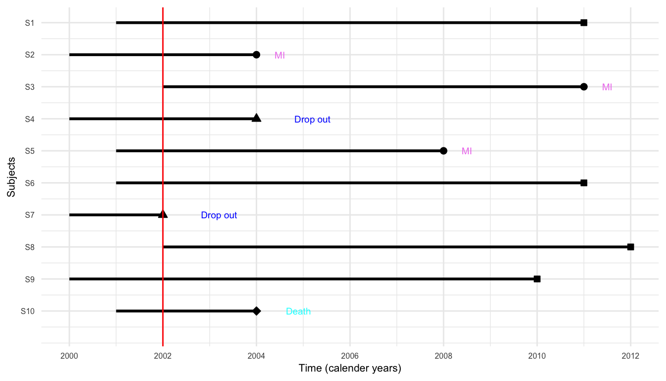
A Hypothetical Study

A hypothetical study

• A small prospective study was run, where 10 participants were recruited to follow

• The event of interest was the development of myocardial infarction (MI, or heart attack) over a period of 10 years (follow-up period)

• Participants are recruited into the study over a period of two years and were then followed for up to 10 years

---

Study in calender years

---

• {S2, S3, S5} $\to$ experienced MI

• {S4, S7} $\to$ dropped out

• {S10} $\to$ died from other causes

• {S1, S6, S8, S9} $\to$ completed 10-year follow-up without MI

---

Study in years

---

---

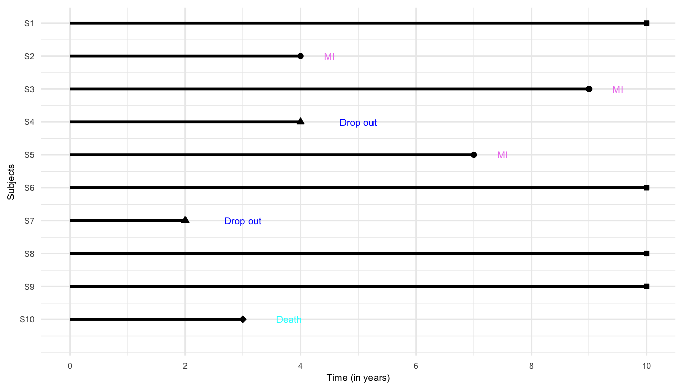
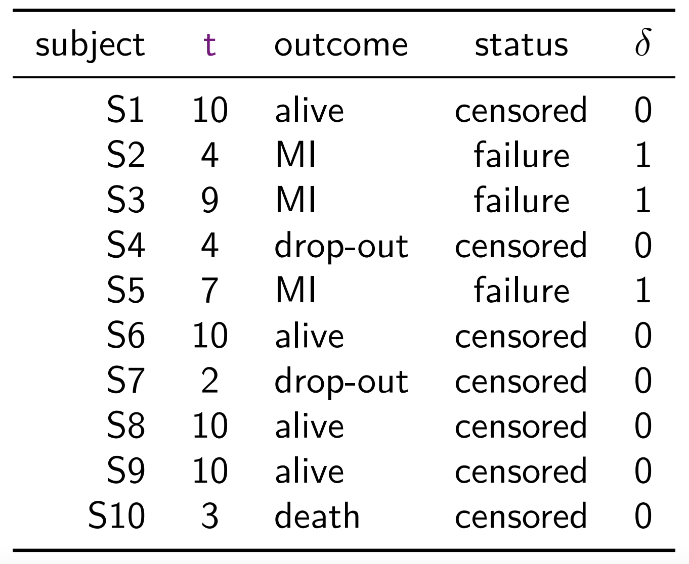
• Times for the subjects who did not experience MI by the end of 10-year follow-up or dropped-out or died from causes not related to MI are known as censored times

• Time-to-MI (time to the event of interest) are known as failure time (or survival time)

• For survival data, the pair (time, status), $(t,\delta )$, is considered as the response

• A sample of survival data can also be expressed as following, where ${}^{+}$ sign indicates censored observations $${10}^{+},4,9,4^{+},7,{10}^{+},2^{+},{10}^{+},{10}^{+},3^{+}$$

2.3 Other type of incomplete data

Acknowledgements

This lecture is adapted from materials created by Mahbub Latif