| time | x |
|---|---|
| 3 | 1 |
| 5 | 0 |
| 8 | 1 |
| 4+ | 1 |
| 10 | 0 |
Chapter 7
(AST405) Lifetime data analysis
7 Semiparametric Multiplicative Hazards Regression Models
7.1 Methods for continuous multiplicative hazards model
Models in which covariates have a multiplicative effect on the hazard function play an important role in the analysis of lifetime data
Proportional hazard (PH) model is one of such models
Depending on whether baseline hazard function is left arbitrary or not, PH model could be either semiparametric or parametric
In this section, semiparametric PH models are discussed, where baseline hazard function is left arbitrary
-
The hazard function is modeled as \[ \begin{aligned} h(t\,\vert\, \mathbf{x}) &= h_0(t)\exp(\mathbf{x}'\boldsymbol{\beta}) \\ &= h_0(t)\exp(\beta_1 x_1 + \beta_2 x_2 + \cdots + \beta_p x_p) \end{aligned} \tag{7.1}\]
-
\(h(t | x)\) = hazard at time t for a person with covariates \(x\)
- \(h_0(t)\) = baseline hazard (unspecified)
- \(\boldsymbol{\beta} = (\beta_1, \ldots, \beta_p)'\;\rightarrow\) vector of regression coefficients
- Covariate vector \(\mathbf{x}\) could include time-varying covariate
- No intercept term is included in \(\mathbf{x}'\boldsymbol{\beta}\)
-
\(h(t | x)\) = hazard at time t for a person with covariates \(x\)
Model (Equation 7.1) is known as “Cox’s proportional hazards model” or simply “Cox model”
No distributional assumption is required for estimating the parameters of the Model (Equation 7.1)
The cumulative baseline hazard function is defined as \[\begin{align} H_0(t) = \int_0^t h_0(u)\,du \end{align}\]
The baseline survivor function \[\begin{align} S_0(t) = \exp\big[-H_0(t)\big] \end{align}\]
The survivor function of \(T\) given covariate vector \(\mathbf{x}\) \[\begin{align} S(t\,\vert\, \mathbf{x}) = \big[S_0(t)\big]^{\exp(\mathbf{x}'\boldsymbol{\beta})} \end{align}\]
Estimation of model parameters
Data \[ \Big\{(t_i, \delta_i, \mathbf{x}_i), i=1, \ldots, n\Big\} \]
Parameters of interest are \(h_0(t)\) and \(\boldsymbol{\beta}\)
Log-likelihood function \[\begin{align} \ell(h_0(t), \boldsymbol{\beta}) & = \log \prod_{i=1}^n \big[f(t_i; \mathbf{x}_i)\big]^{\delta_i}\,\big[S(t_i; \mathbf{x}_i)\big]^{1-\delta_i}\notag\\ & = \sum_i \Big\{\delta_i \log\big[h_0(t_i)\exp(\mathbf{x}_i'\boldsymbol{\beta})\big]+\exp(\mathbf{x}_i'\boldsymbol{\beta})\log S_0(t_i)\Big\}\notag \\ & = \sum_i \Big\{\delta_i \big[\log h_0(t_i) + \mathbf{x}_i'\boldsymbol{\beta}\big] + \exp(\mathbf{x}_i'\boldsymbol{\beta}) \log S_0(t_i)\big]\Big\} \end{align}\]
- No unique solutions of the parameters because the number of parameters to be estimated is greater than the number of observations
Complete likelihood function is not useful for estimating parameters of Cox’s proportional hazards model
There are a number of different likelihood functions defined for estimating parameters, of which Cox’s “partial likelihood function” is widely used for PH models
-
Log-partial-likelihood function is defined as \[\begin{align} \ell_1(\boldsymbol{\beta}) & = \log \prod_{i=1}^n\Bigg(\frac{\exp(\mathbf{x}_i'\boldsymbol{\beta})}{\sum_{k=1}^n Y_k(t_i) \exp(\mathbf{x}_k'\boldsymbol{\beta})}\Bigg)^{\delta_i} \end{align}\]
- \(Y_k(t) = I(t_k \geq t)\,\rightarrow\) indicates whether the \(k\)th subject is still in the risk set at time \(t\) or not
Partial likelihood function can be treated as a regular likelihood function for making statistical inference
For partial likelihood function, the parameters of interest is \(\boldsymbol{\beta}\) and the estimated parameters \[\hat{\boldsymbol{\beta}}={\arg\,\max}_{\boldsymbol{\beta}\in \Theta}\;\ell_1(\boldsymbol{\beta})\] follow asymptotically normal distribution, similar to MLEs
The baseline hazard functions are estimated from the full likelihood function with regression parameters are assumed to be known, i.e. \(\ell(h_0(t), \hat{\boldsymbol{\beta}})\)
- Obtain the expression of partial likelihood function for the following censored sample
7.2 Comparison of two or more lifetime distributions
Let \(S_j(t)\) be the survivor function of lifetime \(T_j\), \(j=1, 2\)
-
Data available \[\{(t_{i}, \delta_{i}, x_i), \,i=1, \ldots, n\}\]
- \(x_i = I(\text{$i$th subject is from group 1})\)
Null hypothesis \[ H_0: S_1(t) = S_2(t) \]
Consider PH model \[ h(t\,\vert\, x) = h_0(t)\exp(\beta x)\;\;\Rightarrow\;\; S(t\,\vert\,x) = [S_0(t)]^{\exp(\beta x)} \]
We can obtain \[\begin{align*} S_2(t) &= S(t\,\vert\, x=0) = S_0(t) \\[.5em] S_1(t) &= S(t\,\vert\, x=1) = [S_0(t)]^{\exp(\beta)}=[S_2(t)]^{\exp(\beta)} \end{align*}\]
The null hypothesis under proportional model assumption \[ H_0: S_1(t) = S_2(t)\;\;\Rightarrow\;\;H_0: \beta=0 \]
Large sample-based property of MLE \(\hat\beta\) can be used to test the null hypothesis
- Log-likelihood function \[\begin{align*} \ell(\beta) &= \log \prod_{i=1}^n \Bigg(\frac{e^{\beta x_i}}{\sum_{k=1}^n Y_k(t_i)\,e^{\beta x_k}}\Bigg)^{\delta_{i}} \\[.25em] &= \sum_{i=1}^n\Big(\delta_i\, x_i\,\beta - \delta_i\log\sum_{k=1}^n Y_k(t_i)\,e^{\beta x_k}\Big) \end{align*}\]
-
Score function \[\begin{align*} U(\beta) &= \sum_{i=1}^n \bigg(\delta_i\,x_i - \frac{\delta_i \sum_{k=1}^n Y_k(t_i)\,e^{\beta x_k}\,x_k}{\sum_{k=1}^n Y_k(t_i)\,e^{\beta x_k}}\bigg)\\[.25em] & = \sum_{i=1}^n\bigg(d_{1i} - \frac{d_i\,n_{1i}\,e^{\beta}}{n_{1i}\,e^{\beta} + n_{2i}} \bigg) \end{align*}\]
\(d_i = \delta_i\)
\(d_{1i} = \delta_i\, x_i = I(\text{$ith$ subject from group 1})\)
\(n_{1i} = \sum_{k=1}^n Y_k(t_i)x_k\,\rightarrow\) number of group 1 subjects at risk at time \(t_i\)
\(n_{2i} = \sum_{k=1}^n Y_k(t_i)(1-x_k)\,\rightarrow\) number of group 2 subjects at risk at time \(t_i\)
- Information matrix \[\begin{align*} I(\beta) &= -\frac{d_i\,n_{1i}\,e^{\beta}n_{1i}\,e^{\beta} - d_i(n_{1i}\,e^{\beta} + n_{2i})n_{1i}\,e^{\beta}}{\big(n_{1i}\,e^{\beta} + n_{2i}\big)^2} \\[.25em] & = \frac{d_i\,n_{1i} n_{2i} e^{\beta}}{\big(n_{1i}\,e^{\beta} + n_{2i}\big)^2} \end{align*}\]
Confidence interval for \(\beta\) can be obtained from the following pivotal quantity \[ Z(\beta) = \frac{U(\beta)}{[I(\beta)]^{1/2}} \] which follows an asymptotic standard normal distribution
\(100(1-\alpha)\%\) confidence interval for \(\beta\) can be obtained from the set of values of \(\beta\) that satisfy \[ Z(\beta)\leq z_{1-\alpha} \]
Under \(H_0: \beta = 0\) \[\begin{align*} U(0) & = \sum_{i=1}^n\bigg(d_{1i} - \frac{d_i\,n_{1i}}{n_{1i} + n_{2i}} \bigg)\\[.25em] I(0) & = \sum_{i=1}^n \frac{d_i\,n_{1i} n_{2i}} {\big(n_{1i} + n_{2i}\big)^2} \end{align*}\]
-
Test statistic \[ Z = \frac{U(0)}{[I(0)]^{1/2}}\sim \mathcal{N}(0, 1) \]
- MLE of \(\beta\) does not require to test \(H_0: \beta=0\) using the statistic \(Z\)
The expression of \(U(0)\) can be considered as the difference between observed number of deaths from group 1, \((d_{1i})\), at time \(t_i\) and the corresponding expected number of deaths \[d_i\times \frac{n_{1i}}{n_{1i} + n_{2i}}\]
At time \(t_i\), there are \(n_i=n_{1i}+n_{2i}\) subjects are at risk and \(d_i\) is either 0 or 1 (i.e. there is no ties in the lifetime)
| group | event | alive | at risk |
|---|---|---|---|
| 1 | \(d_{1i}\) | \(n_{1i} - d_{1i}\) | \(n_{1i}\) |
| 2 | \(d_{2i}\) | \(n_{2i}- d_{2i}\) | \(n_{2i}\) |
| \(d_{i}\) | \(n_i - d_{i}\) | \(n_{i}\) |
- This score test for the Cox model to compare two groups is also known as log-rank test.
Example 7.1.1
Data below show remission times (in weeks) for 40 leukemia patients who were randomly assigned either treatment \(A\) or \(B\)
tab7_1_1# A tibble: 40 × 3
time status group
<dbl> <dbl> <chr>
1 1 1 A
2 3 1 A
3 3 1 A
4 6 1 A
5 7 1 A
6 7 1 A
7 10 1 A
8 12 1 A
9 14 1 A
10 15 1 A
# ℹ 30 more rowssurvdiff(Surv(time, status) ~ group,
data = tab7_1_1) Call:
survdiff(formula = Surv(time, status) ~ group, data = tab7_1_1)
N Observed Expected (O-E)^2/E (O-E)^2/V
group=A 20 17 21.5 0.951 2.36
group=B 20 20 15.5 1.322 2.36
Chisq= 2.4 on 1 degrees of freedom, p= 0.1 coxph(Surv(time, status) ~ group, data = tab7_1_1) %>%
tidy()# A tibble: 1 × 5
term estimate std.error statistic p.value
<chr> <dbl> <dbl> <dbl> <dbl>
1 groupB 0.503 0.332 1.51 0.130Example 7.2.1
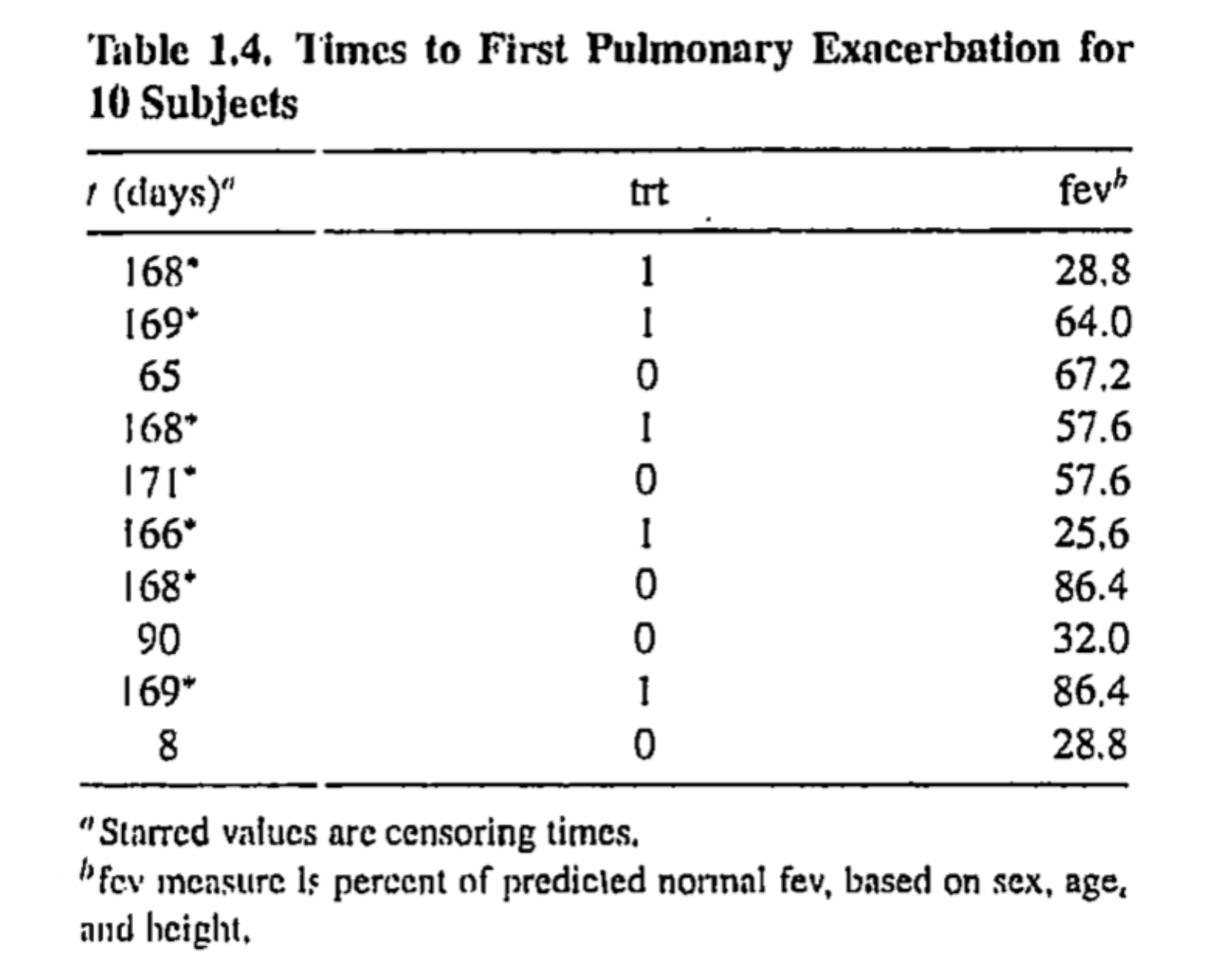
Patients with cystic fibrosis are susceptible to an accumulation of mucus in lungs, which leads to pulmonary exacerbation and deterioration of lung function
-
A clinical trial was conducted to investigate the efficacy of the new drug DNase-1
- Subjects are randomly assigned to a new treatment or a placebo
Time of interest is the time to first exacerbation after randomization and data on fev (forced expiatory volume at the time of randomization) are also measured
Creating the data from the R object rhDNase
tab1_4 <- as_tibble(rhDNase) %>%
  filter(is.na(ivstart) | ivstart > 0) %>%
  mutate(time0 = as.numeric(end.dt - entry.dt),
         status = as.numeric(!is.na(ivstart)),
         time = if_else(status == 1, ivstart, time0),
         fevm = fev - mean(fev)) %>%
  group_by(id) %>%
  mutate(visit = n()) %>%
  ungroup()
Cox’s PH model \[ h(t\,\vert\, \text{trt, fevm}) = h_0(t)\exp(\beta_1\,\text{trt} + \beta_2\, \text{fevm}) \] R code for fitting the model
mod1 <- coxph(Surv(time,  status) ~ trt + fevm,
              data = tab1_4)
Estimates of regression coefficients
tidy(mod1)# A tibble: 2 × 5
term estimate std.error statistic p.value
<chr> <dbl> <dbl> <dbl> <dbl>
1 trt -0.352 0.106 -3.31 9.47e- 4
2 fevm -0.0188 0.00226 -8.31 9.63e-17Treatment group patients have lower hazard for time to first exacerbation
As FEV value increases the hazard of first exacerbation decreases
Effects of treatment and FEV are significant on the hazard of first exacerbation decreases
| term | estimate | p.value | HR | 2.5 % | 97.5 % |
|---|---|---|---|---|---|
| trt | -0.352 | 0.001 | 0.703 | 0.571 | 0.867 |
| fevm | -0.019 | 0.000 | 0.981 | 0.977 | 0.986 |
Treatment group patients have about \(30\)% lower hazard of first exacerbation than that of the placebo group patients provided FEV value remains constant
For 1-unit increase of FEV value, hazard of first exacerbation decreases about \(2\)% provided treatment group remains constant
survfit() provides estimate of survivor function and corresponding standard errors
tidy(survfit(mod1)) %>%
    as_tibble()
# A tibble: 161 × 8
time n.risk n.event n.censor estimate std.error conf.high conf.low
<dbl> <dbl> <dbl> <dbl> <dbl> <dbl> <dbl> <dbl>
1 1 761 1 0 0.999 0.00138 1 0.996
2 5 760 3 0 0.994 0.00277 1.00 0.989
3 6 757 1 0 0.993 0.00311 0.999 0.987
4 8 756 4 0 0.988 0.00420 0.996 0.979
5 9 752 3 0 0.983 0.00489 0.993 0.974
6 11 749 2 0 0.981 0.00530 0.991 0.971
7 13 747 2 0 0.978 0.00569 0.989 0.967
8 14 745 2 0 0.975 0.00606 0.987 0.964
9 15 743 4 0 0.970 0.00675 0.983 0.957
10 16 739 2 0 0.967 0.00708 0.980 0.953
# ℹ 151 more rows