{survival} package

(AST405) Lifetime data analysis

Author

Md Rasel Biswas

Time-to-event data

Time-to-event data are defined as ${(t_{i}, δ_{i}), i = 1, \dots, n}$
- $t_{i} \to$ observed time
- $δ_{i} \to$ censoring indicator (1=failure, 0=censored)

Defining time and censoring indicator in R for the following sample of five observations $20, 13^{+}, 10, 25, 18^{+}$

dat0 <- tibble(
  time = c(20, 13, 10, 25, 18),
  status = c(1, 0, 1, 1, 0)
)

dat0

# A tibble: 5 × 2
   time status
  <dbl>  <dbl>
1    20      1
2    13      0
3    10      1
4    25      1
5    18      0

`survival` package

There are a number of R packages available for analyzing time-to-event data
The survival package will be used for the course, the current (January 2025) version of survival package is 3.8-3
Author, contributors, and maintainer of survival package
- Terry M Therneau [aut, cre]
- Thomas Lumley
- Atkinson Elizabeth
- Crowson Cynthia

Creating survival objects and curves

survival::survfit() function is used to obtain non-parametric estimate survivor function

survfit(Surv(time, time2, event) ~ x, data)

Surv $\to$ creates a survival object, which has arguments such as, time, time2, event, and type (censoring type “right”, “left”, “interval”, etc.)
time $\to$ observed time (numeric object)
event $\to$ censoring status (1=failure, 0=censored)
x $\to$ strata (categorical variable), x=1 when stratified analysis is not required (single curve)

Some important arguments of survfit() function
- stype $\to$ 1 (direct estimation of survivor function), 2 (survivor function estimated from cumulative hazard function)
- ctype $\to$ method used to estimate cumulative hazard function (1=Nelson Aalen, 2=Fleming-Harrington)
- conf.type $\to$ available options include (“none”, “plain”, “log” (default), “log-log”, and “logit”)

Example

mp6 <- c(6, 6, 6, 6, 7, 9, 10, 10, 11, 13, 16, 17,
             19, 20, 22, 23, 25, 32, 32, 34, 35)
plc <- c(1, 1, 2, 2, 3, 4, 4, 5, 5, 8, 8, 8, 8,
         11, 11, 12, 12, 15, 17, 22, 23)
gehan65 <- tibble(
  time = c(mp6, plc),
  status = c(1, 1, 1, 0, 1, 0, 1, 0, 0, 1, 1, 0, 0,
             0, 1, 1, rep(0, 5), rep(1, 21)),
  drug = c(rep("6-MP", 21), rep("placebo", 21))
)
glimpse(gehan65)

Rows: 42
Columns: 3
$ time   <dbl> 6, 6, 6, 6, 7, 9, 10, 10, 11, 13, 16, 17, 19, 20, 22, 23, 25, 3…
$ status <dbl> 1, 1, 1, 0, 1, 0, 1, 0, 0, 1, 1, 0, 0, 0, 1, 1, 0, 0, 0, 0, 0, …
$ drug   <chr> "6-MP", "6-MP", "6-MP", "6-MP", "6-MP", "6-MP", "6-MP", "6-MP",…

gehan65 %>% 
  count(drug, status)

# A tibble: 3 × 3
  drug    status     n
  <chr>    <dbl> <int>
1 6-MP         0    12
2 6-MP         1     9
3 placebo      1    21

No censored time for Placebo group.

# keep only the Treatment Group
dat6MP <- gehan65 %>% 
  filter(drug == "6-MP")

# Fitting model for the Treatment Group without any covariate
mod1 <- survfit(Surv(time = time, event = status) ~ 1, 
                conf.type = "plain",
                data = dat6MP)

Default conf.type is log

# Produces summary of the KM fit
summary(mod1)

Call: survfit(formula = Surv(time = time, event = status) ~ 1, data = dat6MP, 
    conf.type = "plain")

 time n.risk n.event survival std.err lower 95% CI upper 95% CI
    6     21       3    0.857  0.0764        0.707        1.000
    7     17       1    0.807  0.0869        0.636        0.977
   10     15       1    0.753  0.0963        0.564        0.942
   13     12       1    0.690  0.1068        0.481        0.900
   16     11       1    0.627  0.1141        0.404        0.851
   22      7       1    0.538  0.1282        0.286        0.789
   23      6       1    0.448  0.1346        0.184        0.712

Kaplan-Meier plots

# This produces the KM plot; but it is not nice.
plot(mod1)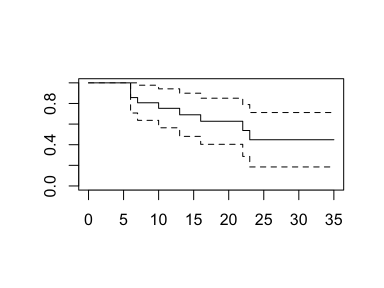

We’ll use the ggplot2 package for nicer plots.

broom::tidy(mod1)

# A tibble: 16 × 8
    time n.risk n.event n.censor estimate std.error conf.high conf.low
   <dbl>  <dbl>   <dbl>    <dbl>    <dbl>     <dbl>     <dbl>    <dbl>
 1     6     21       3        1    0.857    0.0891     1        0.707
 2     7     17       1        0    0.807    0.108      0.977    0.636
 3     9     16       0        1    0.807    0.108      0.977    0.636
 4    10     15       1        1    0.753    0.128      0.942    0.564
 5    11     13       0        1    0.753    0.128      0.942    0.564
 6    13     12       1        0    0.690    0.155      0.900    0.481
 7    16     11       1        0    0.627    0.182      0.851    0.404
 8    17     10       0        1    0.627    0.182      0.851    0.404
 9    19      9       0        1    0.627    0.182      0.851    0.404
10    20      8       0        1    0.627    0.182      0.851    0.404
11    22      7       1        0    0.538    0.238      0.789    0.286
12    23      6       1        0    0.448    0.300      0.712    0.184
13    25      5       0        1    0.448    0.300      0.712    0.184
14    32      4       0        2    0.448    0.300      0.712    0.184
15    34      2       0        1    0.448    0.300      0.712    0.184
16    35      1       0        1    0.448    0.300      0.712    0.184

broom::tidy(mod1) %>% 
  ggplot() +
  geom_step(aes(time, estimate))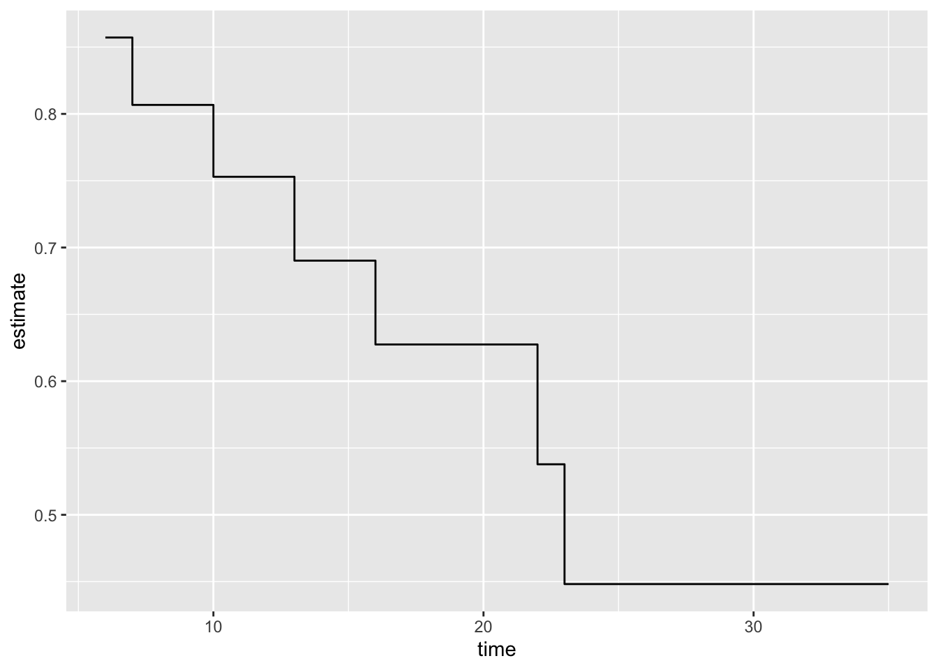

tidy(mod1) %>% 
  ggplot() +
  geom_step(aes(time, estimate)) + 
  geom_step(aes(time, conf.high), linetype = "dotted", col = "red") +
  geom_step(aes(time, conf.low), linetype = "dotted", col = "red")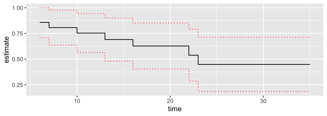

Estimating survival probability

To estimate the probability of survival time, we use summary() with the times argument.

summary(mod1, times = 10)

Call: survfit(formula = Surv(time = time, event = status) ~ 1, data = dat6MP, 
    conf.type = "plain")

 time n.risk n.event survival std.err lower 95% CI upper 95% CI
   10     15       5    0.753  0.0963        0.564        0.942

So the probability of surviving to 10 years is 0.75.

We can produce nice publication-ready tables of survival probability estimates using the tbl_survfit() function from the gtsummary package

mod1 |> 
  gtsummary::tbl_survfit(
    times = 10,
    label_header = "**10-year survival (95% CI)**"
  )

Characteristic	10-year survival (95% CI)
Overall	75% (56%, 94%)

Estimating quantiles

quantile(mod1, probs = c(0.20, 0.25, 0.50, 0.75, 0.80))

$quantile
20 25 50 75 80 
10 13 23 NA NA 

$lower
20 25 50 75 80 
 6  6 13 23 23 

$upper
20 25 50 75 80 
22 23 NA NA NA

So, first quartile is 13. Median is 23.

We can produce nice publication-ready tables of median survival time estimates using the tbl_survfit() function from the gtsummary package

mod1 %>% 
  gtsummary::tbl_survfit(
    probs = 0.5,
    label_header = "**Median survival (95% CI)**"
  )

Characteristic	Median survival (95% CI)
Overall	23 (13, —)

Fitting model with a covariate

mod2 <- survfit(
  Surv(time = time, event = status) ~ drug,
  data = gehan65,
  conf.type = "plain"
  )

broom::tidy(mod2)

# A tibble: 28 × 9
    time n.risk n.event n.censor estimate std.error conf.high conf.low strata   
   <dbl>  <dbl>   <dbl>    <dbl>    <dbl>     <dbl>     <dbl>    <dbl> <chr>    
 1     6     21       3        1    0.857    0.0891     1        0.707 drug=6-MP
 2     7     17       1        0    0.807    0.108      0.977    0.636 drug=6-MP
 3     9     16       0        1    0.807    0.108      0.977    0.636 drug=6-MP
 4    10     15       1        1    0.753    0.128      0.942    0.564 drug=6-MP
 5    11     13       0        1    0.753    0.128      0.942    0.564 drug=6-MP
 6    13     12       1        0    0.690    0.155      0.900    0.481 drug=6-MP
 7    16     11       1        0    0.627    0.182      0.851    0.404 drug=6-MP
 8    17     10       0        1    0.627    0.182      0.851    0.404 drug=6-MP
 9    19      9       0        1    0.627    0.182      0.851    0.404 drug=6-MP
10    20      8       0        1    0.627    0.182      0.851    0.404 drug=6-MP
# ℹ 18 more rows

broom::tidy(mod2) %>% 
  select(time, estimate, strata)

# A tibble: 28 × 3
    time estimate strata   
   <dbl>    <dbl> <chr>    
 1     6    0.857 drug=6-MP
 2     7    0.807 drug=6-MP
 3     9    0.807 drug=6-MP
 4    10    0.753 drug=6-MP
 5    11    0.753 drug=6-MP
 6    13    0.690 drug=6-MP
 7    16    0.627 drug=6-MP
 8    17    0.627 drug=6-MP
 9    19    0.627 drug=6-MP
10    20    0.627 drug=6-MP
# ℹ 18 more rows

broom::tidy(mod2) %>% 
  ggplot() + 
  geom_step(aes(time, estimate, col = strata))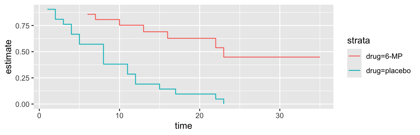

mod2 %>% 
  gtsummary::tbl_survfit(
    times = 10,
    label_header = "**10-year survival (95% CI)**"
  )

Characteristic	10-year survival (95% CI)
drug
6-MP	75% (56%, 94%)
placebo	38% (17%, 59%)

mod2 %>% 
  gtsummary::tbl_survfit(
    probs = 0.5,
    label_header = "**Median survival (95% CI)**"
  )

Characteristic	Median survival (95% CI)
drug
6-MP	23 (13, —)
placebo	8.0 (4.0, 11)

Time-to-event data

survival package

Creating survival objects and curves

Example

Kaplan-Meier plots

Estimating survival probability

Estimating quantiles

Fitting model with a covariate

`survival` package