Chapter 4

(AST405) Lifetime data analysis

4 Inference procedures for parametric models

Introduction

• Likelihood methods for lifetime data were introduced in Chapter 2, which includes derivation of likelihood function for different types of censored data

  • Maximum likelihood estimator

  • Inference about parameters (hypothesis testing and confidence intervals)

Likelihood function (Complete data)

• Let $t_1,\dots ,t_n$ be a random sample from a distribution $f(t;\mathit{\theta })$, where $\mathit{\theta }$ is a $p$-dimensional vector of parameters

• Likelihood and log-likelihood function $$\begin{array}{rl}L(\mathit{\theta })& =\prod _{i=1}^{n}f(t_i;\theta )\\ \ell (\mathit{\theta })=\log L(\mathit{\theta })& =\sum _{i=1}^n\log f(t_i;\mathit{\theta })\end{array}$$

• Maximum likelihood estimator (MLE) $$\begin{array}{r}\hat{\mathit{\theta }}={argmax}_{\mathit{\theta }\in \mathrm{\Theta }}\ell (\mathit{\theta })\end{array}$$

Statistical inference (Complete data)

• Large sample property of MLE $$\begin{array}{r}\hat{\mathit{\theta }}\sim \mathcal{N}(\mathit{\theta },[\mathcal{I}(\mathit{\theta }){]}^{-1})\end{array}$$

  • Fisher expected information matrix $$\begin{array}{r}\mathcal{I}(\mathit{\theta })=E[-\frac{{\partial }^2\ell (\mathit{\theta })}{\partial \mathit{\theta }\partial {\mathit{\theta }}^{\prime }}]\end{array}$$

  • Observed information matrix $$\begin{array}{r}I(\hat{\mathit{\theta }})=-\frac{{\partial }^2\ell (\mathit{\theta })}{\partial \mathit{\theta }\partial {\mathit{\theta }}^{\prime }}{|}_{\mathit{\theta }=\hat{\mathit{\theta }}}\end{array}$$

Likelihood function (Type I or random censoring)

• Data: $\{(t_i,{\delta }_i),i=1,\dots ,n\}$

  • $t_i$ is a sample realization of ${\tilde{T}}_i=min(T_i,C_i)$

  • lifetime $T_i$ follows a distribution with pdf $f(t_i;\mathit{\theta })$ and the corresponding survivor function $S(t_i;\mathit{\theta })$

  • censoring time $C_i$ could be random or fixed depending on the censoring mechanism

  • ${\delta }_i=I(T_i\le C_i)$, censoring indicator

---

• Data for type I or random censoring $$\{(t_i,{\delta }_i),i=1,\dots ,n\}$$

• Likelihood function $$\begin{array}{rl}L(\mathit{\theta })& =\prod _{i=1}^n[f(t_i;\mathit{\theta }{]}^{{\delta }_i}[S(t_i;\mathit{\theta }){]}^{1-{\delta }_i}\\ & =\prod _{i=1}^n[S(t_i;\mathit{\theta })h(t_i;\mathit{\theta }){]}^{{\delta }_i}[S(t_i;\mathit{\theta }){]}^{1-{\delta }_i}\\ & =\prod _{i=1}^n[S(t_i;\mathit{\theta }][h(t_i;\mathit{\theta }){]}^{{\delta }_i}\end{array}$$

Likelihood function (Type II censoring)

• Let lifetime $T_i$ $(i=1,\dots ,n)$ follows a distribution with pdf $f(t_i;\mathit{\theta })$ and the corresponding survivor function $S(t_i;\mathit{\theta })$

• The experiment was terminated after observing $r$ smallest lifetimes
  $$t_{(1)}⩽\cdots ⩽t_{(r)}$$

• The remaining $(n-r)$ observations are considered as censored at $t_{(r)}$

• Likelihood function $$\begin{array}{r}L(\mathit{\theta })=[\prod _{i=1}^{r}f(t_{(i)};\mathit{\theta })][S(t_{(r)};\mathit{\theta }){]}^{n-r}\end{array}$$

Statistical inference (censored sample)

• For censored samples, the result “asymptotic distribution of MLE is normal” is still valid

• The expression of the Fisher expected information matrix $\mathcal{I}(\mathit{\theta })$ is complex for censored data, observed information matrix $I(\hat{\theta })$ is used in making inference with censored sample

4.1 Exponential distribution

• The exponential distribution is the first lifetime model for which statistical methodology were extensively developed

• Exact tests can be developed for exponential distribution for certain type of censoring mechanism

• Exponential distribution assume constant hazard and its use is limited for analyzing real life problems

---

• Probability density function $$\begin{array}{r}f(t;\theta )=(1/\theta )\exp (-t/\theta )t⩾0,\theta >0\end{array}$$

• Hazard function $$\begin{array}{r}h(t;\theta )=(1/\theta )\end{array}$$

• Survivor function $$\begin{array}{r}S(t;\theta )=\exp (-t/\theta )\end{array}$$

• $p$th quantile $$S(t_p;\theta )=1-p\Rightarrow \exp (-t_p;\theta )=1-p\Rightarrow t_p=-\theta \log (1-p)$$

---

Homework

• Estimation and related inference of exponential distribution when the sample has no censored observations

Type I or random censoring

• Lifetime $T\sim \text{Exp}(\theta )$, $\theta >0$

• Data: $\{(t_i,{\delta }_i),i=1,\dots ,n\}$

• Likelihood function $$\begin{array}{rl}L(\theta )& =\prod _{i=1}^n[f(t_i;\theta ){]}^{{\delta }_i}[S(t_i;\theta ){]}^{1-{\delta }_i}\\ & =\prod _{i=1}^{n}S(t_i;\theta )[h(t_i;\theta ){]}^{{\delta }_i}\\ & =\prod _{i=1}^n\exp (-t_i/\theta )(1/\theta {)}^{{\delta }_i}\end{array}$$

---

• Likelihood function $$\begin{array}{rl}L(\theta )& =\prod _{i=1}^n\exp (-t_i/\theta )(1/\theta {)}^{{\delta }_i}\end{array}$$

• Log-likelihood function $$\begin{array}{rl}\ell (\theta )& =\sum _{i=1}^n[-(t_i/\theta )-{\delta }_i\log (\theta )]\\ & =-\frac{1}{\theta }\sum _i{t}_i-r\log (\theta )\end{array}$$

  • $r=\sum _i{\delta }_i\to$ the number of failures observed in the sample

---

• Log-likelihood function $$\begin{array}{rl}\ell (\theta )& =-\frac{1}{\theta }\sum _i{t}_i-r\log (\theta )\end{array}$$

• MLE $$\frac{\partial \ell (\theta )}{\partial \theta }{|}_{\theta =\hat{\theta }}=0\Rightarrow \frac{1}{{\hat{\theta }}^2}\sum _i{t}_i-\frac{r}{\hat{\theta }}=0$$ $$\begin{array}{r}\hat{\theta }=\sum _{i=1}^n{t}_i/r\end{array}$$

  • Assuming $r>0$ and no finite MLE exist for $r=0$

---

• Information matrix

$$\begin{array}{rl}I(\theta )& =-\frac{{\partial }^2\ell (\theta )}{\partial {\theta }^2}\\ & =-\frac{\partial }{\partial \theta }[\frac{1}{{\theta }^2}\sum _i{t}_i-\frac{r}{\theta }]\\ & =\frac{2}{{\theta }^3}\sum _i{t}_i-\frac{r}{{\theta }^2}\end{array}$$

• Replacing the parameter $\theta$ by its MLE $\hat{\theta }=\sum _i{t}_i/r$, the observed information matrix becomes $$I(\hat{\theta })=\frac{r}{{\hat{\theta }}^2}$$

Confidence interval (Method I)

• Using $\hat{\theta }$’s asymptotic distribution $$\begin{array}{r}{Z}_1=\frac{\theta -\hat{\theta }}{[I(\hat{\theta }){]}^{-1/2}}=\frac{\theta -\hat{\theta }}{\hat{\theta }/\sqrt{r}}\sim \mathcal{N}(0,1)\end{array}$$

• For a small sample, $Z_1$ does not approximate the standard normal distribution very accurately

• For a sample with a small number of uncensored observations, $\ell (\theta )$ tends to be asymmetric

Confidence interval (Method II)

• Sprott (1980) showed that ${\ell }_1(\varphi )=\ell ({\varphi }^{-3})$ is more closer to symmetric compared to $\ell (\theta )$, where $\varphi ={\theta }^{-1/3}\Rightarrow {\varphi }^3=1/\theta$ $$\begin{array}{rl}\ell (\theta )& =-(1/\theta )\sum _i{t}_i-r\log \theta \\ {\ell }_1(\varphi )& =-{\varphi }^3\sum _i{t}_i+3r\log (\varphi )\end{array}$$

  • MLE $\hat{\varphi }={\hat{\theta }}^{-1/3}=[\sum _i{t}_i/r{]}^{-1/3}$

  • Observed information matrix $$\begin{array}{r}{I}_1(\varphi )=6\varphi \sum _i{t}_i+\frac{3r}{{\varphi }^2}\Rightarrow I_1(\hat{\varphi })=\frac{9r}{{\hat{\varphi }}^2}\end{array}$$

---

• Pivotal quantity $$Z_2=\frac{\varphi -\hat{\varphi }}{[I_1(\hat{\varphi }){]}^{-1/2}}=\frac{\varphi -\hat{\varphi }}{\hat{\varphi }/\sqrt{9r}}\sim \mathcal{N}(0,1)$$

  • Approximation of $Z_2$ is quite accurate compared to that of $Z_1$

Confidence interval (Method III)

• Likelihood ratio statistic $\mathrm{\Lambda }(\theta )=2\ell (\hat{\theta })-2\ell (\theta )$ can also be used to obtain confidence interval for $\theta$, where $$\begin{array}{rl}\ell (\theta )& =-(1/\theta )\sum _i{t}_i-r\log (\theta )\\ & =-r(\hat{\theta }/\theta )-r\log (\theta )\\ \ell (\hat{\theta })& =-(1/\hat{\theta })\sum _i{t}_i-r\log (\hat{\theta })\\ & =-r-r\log (\hat{\theta })\end{array}$$

---

• LRT statistic $$\begin{array}{rl}\mathrm{\Lambda }(\theta )& =2\ell (\hat{\theta })-2\ell (\theta )\\ & =2r[(\hat{\theta }/\theta )-1+\log (\theta /\hat{\theta })]\end{array}$$

• Two-sided $(1-\alpha )100\mathrm{\%}$ confidence intervals are obtained as the set of $\theta$ values that satisfy $$\mathrm{\Lambda }(\theta )\le {\chi }_{(1),1-\alpha }^2$$

Confidence interval of survivor function

• Confidence interval for the parameter $\theta$ can also be used to obtain confidence intervals for a monotone function of $\theta$, such as $$S(t;\theta )=\exp (-t/\theta )\text{or}h(t;\theta )=1/\theta$$

• Let $100(1-\alpha )\mathrm{\%}$ confidence interval for $\theta$ $$L(\text{Data})⩽\theta ⩽U(\text{Data}),$$ where $\text{Data}=\{(t_i,{\delta }_i),i=1,\dots ,n\}$

---

• $100(1-\alpha )\mathrm{\%}$ confidence interval for $S(t_0;\theta )=\exp (-t_0/\theta )$ $$\begin{array}{rl}L(\text{Data})& ⩽\theta ⩽U(\text{Data})\\ t_0/U(\text{Data})& ⩽(t_0/\theta )⩽t_0/L(\text{Data})\\ -t_0/L(\text{Data})& ⩽(-t_0/\theta )⩽-t_0/U(\text{Data})\\ \exp (-t_0/L(\text{Data}))& ⩽S(t_0;\theta )⩽\exp (-t_0/U(\text{Data}))\end{array}$$

Confidence interval of hazard function

• $100(1-\alpha )\mathrm{\%}$ confidence interval for $h(t_0;\theta )=1/\theta$ $$(1/U(\text{Data}))⩽h(t_0;\theta )⩽(1/L(\text{Data}))$$

Example 4.1.1

• Lifetimes (in days) of 10 pieces of equipment

time	status
2	1
72	0
51	1
60	0
33	1
27	1
14	1
24	1
4	1
21	0

• Assume lifetimes follow exponential distribution with parameter, i.e. $T_i\sim \text{Exp}(\theta )$

---

• MLE $$\hat{\theta }=\frac{\sum _i{t}_i}{r}=\frac{308}{7}=44.0$$

• 95% confidence interval of $\theta$ (Method I)

$$\begin{array}{rl}\hat{\theta }\pm z_{.975}[I(\hat{\theta }){]}^{-1/2}& \Rightarrow \hat{\theta }\pm z_{.975}(\hat{\theta }/\sqrt{r})\\ & \Rightarrow 44.0\pm (1.96)(44.0/\sqrt{7})\\ & \Rightarrow 11.4⩽\theta ⩽76.6\end{array}$$

---

• 95% confidence interval of $\theta$ (Method II)

  • $\hat{\varphi }={\hat{\theta }}^{-1/3}=(44.0{)}^{-1/3}=0.283$

  • Confidence interval for $\varphi$
    $$\begin{array}{rl}\hat{\varphi }\pm z_{.975}[I_1(\hat{\varphi }){]}^{-1/2}& \Rightarrow \hat{\varphi }\pm z_{.975}(\hat{\varphi }/\sqrt{9r})\\ & \Rightarrow 0.28\pm (1.96)(0.28/\sqrt{63})\\ & \Rightarrow 0.21⩽\varphi ⩽0.35\end{array}$$

  • Confidence interval for $\theta$

$$\begin{array}{rl}0.21⩽\varphi ⩽0.35& \Rightarrow 0.21⩽{\theta }^{-1/3}⩽0.35\\ & \Rightarrow (0.35{)}^{-3}⩽\theta ⩽(0.21{)}^{-3}\\ & \Rightarrow 22.69⩽\theta ⩽103.03\end{array}$$

---

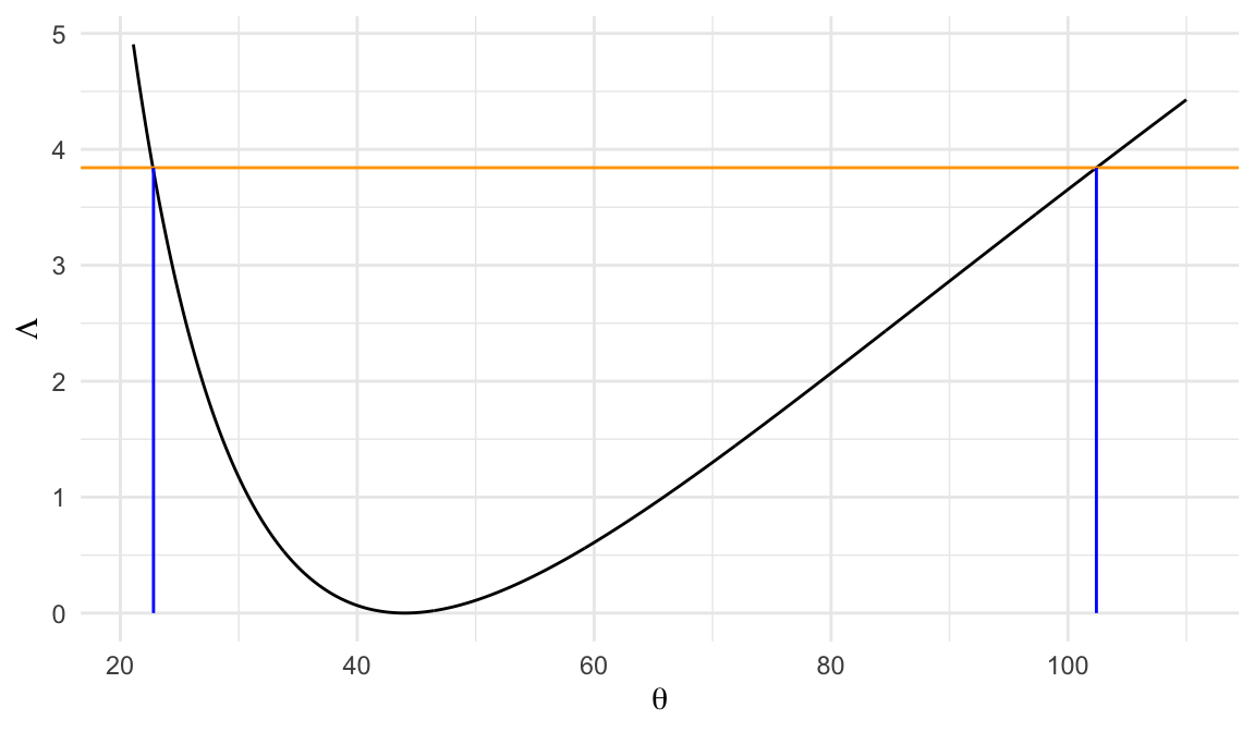
• Likelihood ratio statistic $$\mathrm{\Lambda }(\theta )=2r[(\hat{\theta }/\theta )-1-\log (\hat{\theta }/\theta )]$$

  • 95% CI for $\theta$ can be obtained from the set of $\theta$’s such that $$\mathrm{\Lambda }(\theta )\le {\chi }_{(1),.95}^2=3.84$$

  • 95% CI for $\theta$ $$22.8\text{to}102.4$$

---

---

A comparison of 95% CI for $\theta$ with the data on lifetimes of 10 pieces of equipment (Example 4.1.1)

method	lower	upper
Normal approx.	11.40	76.60
Sprott	22.69	103.03
LRT	22.80	102.40

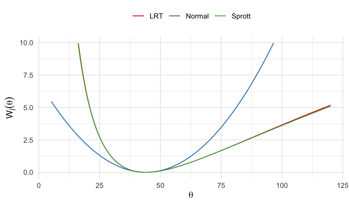
Methods for CI

• Normal approximation $$W_1(\theta )=[\frac{(\hat{\theta }-\theta )}{[I(\hat{\theta }){]}^{-1/2}}{]}^2=(\hat{\theta }-\theta {)}^{2}I(\hat{\theta })$$

• Sprott’s method $$W_2(\theta )=[\frac{(\hat{\varphi }-\varphi )}{[I_1(\hat{\varphi }){]}^{-1/2}}{]}^2=({\hat{\theta }}^{-1/3}-{\theta }^{-1/3}{)}^2{I}_1({\hat{\theta }}^{-1/3})$$

• LRT $$W_3(\theta )=2\ell (\hat{\theta })-2\ell (\theta )=2r[(\hat{\theta }/\theta )-1-\log (\hat{\theta }/\theta )]$$

• $W_j(\theta )\sim {\chi }_{(1)}^{2}j=1,2,3\text{under }{H}_0$

Comparisons between normal approximations and LRT

Type II censoring plan

• Assume lifetime $T\sim \text{Exp}(\theta )$

• Let $t_{(1)}<\cdots <t_{(r)}$ be the $r$ smallest lifetimes observed from an experiment with $n(\ge r)$ subjects

• The joint distribution of $t_{(1)},\dots ,t_{(r)}$ $$\begin{array}{rl}{f}_T(t_{(1)},\dots ,t_{(r)})& =\frac{n!}{(n-r)!}[\prod _{i=1}^r(1/\theta )e^{-t_{(i)}/\theta }][e^{-t_{(r)}/\theta )}{]}^{n-r}\\ & =\frac{n!}{(n-r)!}(1/\theta {)}^r{e}^{-\frac{1}{\theta }[\sum _{i=1}^r{t}_{(i)}+(n-r)t_{(r)}]}\\ & =\frac{n!}{(n-r)!}(1/\theta {)}^r{e}^{-T_0/\theta }\end{array}$$

---

• The log-likelihood function $$\begin{array}{rl}\ell (\theta )& =-\frac{1}{\theta }\sum _i{t}_{(i)}-r\log (\theta )-(1/\theta )(n-r)t_{(r)}+\text{Const.}\\ & =-\frac{1}{\theta }[\sum _{i=1}^r{t}_{(i)}+(n-r)t_{(r)}]-r\log (\theta )+\text{Const.}\\ & =-\frac{T_0}{\theta }-r\log (\theta )+\text{Const.}\end{array}$$

---

• Maximum likelihood estimator $$\frac{\partial \ell (\theta )}{\partial \theta }{|}_{\theta =\hat{\theta }}=0\Rightarrow \hat{\theta }=(1/r)[\sum _{i=1}^r{t}_{(i)}+(n-r)t_{(r)}]$$

  • Observed information matrix $$I(\hat{\theta })=\frac{-{\partial }^2\ell (\theta )}{\partial {\theta }^2}{|}_{\theta =\hat{\theta }}=\frac{r}{{\hat{\theta }}^2}$$

• $(1-\alpha )100\mathrm{\%}$ CI for $\theta$ (by Normal approximation) $$\begin{array}{r}\hat{\theta }\pm z_{1-\alpha /2}[I(\hat{\theta }){]}^{-1/2}\end{array}$$

Exact confidence interval

• Exact confidence interval for $\theta$ can be derived for uncensored and Type II censored samples, define $$\begin{array}{rl}{W}_1& =n{t}_{(1)}\\ W_2& =(n-1)(t_{(2)}-t_{(1)})\\ ⋮& \\ W_r& =(n-r+1)(t_{(r)}-t_{(r-1)})\end{array}$$

• In general $$W_i=(n-i+1)(t_{(i)}-t_{(i-1)})i=1,\dots ,r$$

---

• It can be shown that $$\begin{array}{}\text{(4.1)}& \sum _{i=1}^r{W}_i=\sum _{i=1}^r{t}_{(i)}+(n-r)t_{(r)}=T_0\end{array}$$

---

• The joint distribution of $W_1=g_1(t_{(1)},\dots ,t_{(r)}),\dots ,W_r=g_r(t_{(1)},\dots ,t_{(r)})$ $$\begin{array}{r}{f}_W(w_1,\dots ,w_r)=f_T(g_1^{-1}(w_1,\dots ,w_r),\dots ,g_r^{-1}(w_1,\dots ,w_r))|J|\end{array}$$ where $$\begin{array}{rl}J& =\frac{\partial (g_1^{-1}(w_1,\dots ,w_r),\dots ,g_r^{-1}(w_1,\dots ,w_r))}{\partial (w_1,\dots ,w_r)}\\ & =\left[\begin{array}{cccc}\frac{\partial g_1^{-1}(w_1,\dots ,w_r)}{\partial w_1}& \frac{\partial g_2^{-1}(w_1,\dots ,w_r)}{\partial w_1}& \cdots & \frac{\partial g_r^{-1}(w_1,\dots ,w_r)}{\partial w_1}\\ \frac{\partial g_1^{-1}(w_1,\dots ,w_r)}{\partial w_2}& \frac{\partial g_2^{-1}(w_1,\dots ,w_r)}{\partial w_2}& \cdots & \frac{\partial g_r^{-1}(w_1,\dots ,w_r)}{\partial w_2}\\ ⋮& ⋮& \ddots & ⋮\\ \frac{\partial g_1^{-1}(w_1,\dots ,w_r)}{\partial w_r}& \frac{\partial g_2^{-1}(w_1,\dots ,w_r)}{\partial w_r}& \cdots & \frac{\partial g_r^{-1}(w_1,\dots ,w_r)}{\partial w_r}\end{array}\right]\end{array}$$

---

$$\begin{array}{rl}{w}_1& =g_1(t_{(1)},\dots ,t_{(r)})=n{t}_{(1)}\Rightarrow t_{(1)}=g_1^{-1}(w_1,\dots ,w_r)=\frac{w_1}{n}\\ w_2& =g_2(t_{(1)},\dots ,t_{(r)})=(n-1)(t_{(2)}-t_{(1)})\\ & \Rightarrow t_{(2)}=g_2^{-1}(w_1,\dots ,w_r)=\frac{w_2}{n-1}+\frac{w_1}{n}\\ ⋮& \\ w_r& =g_r(t_{(1)},\dots ,t_{(r)})=(n-r+1)(t_{(r)}-t_{(r-1)})\\ & \Rightarrow t_{(r)}=g_r^{-1}(w_1,\dots ,w_r)=\frac{w_r}{n-r+1}+\cdots +\frac{w_2}{n-1}+\frac{w_1}{n}\end{array}$$

---

$$\begin{array}{rl}J& =\left[\begin{array}{cccc}\frac{\partial g_1^{-1}(w_1,\dots ,w_r)}{\partial w_1}& \frac{\partial g_2^{-1}(w_1,\dots ,w_r)}{\partial w_1}& \cdots & \frac{\partial g_r^{-1}(w_1,\dots ,w_r)}{\partial w_1}\\ \frac{\partial g_1^{-1}(w_1,\dots ,w_r)}{\partial w_2}& \frac{\partial g_2^{-1}(w_1,\dots ,w_r)}{\partial w_2}& \cdots & \frac{\partial g_r^{-1}(w_{!},\dots ,w_r)}{\partial w_2}\\ ⋮& ⋮& \ddots & ⋮\\ \frac{\partial g_1^{-1}(w_1,\dots ,w_r)}{\partial w_r}& \frac{\partial g_2^{-1}(w_1,\dots ,w_r)}{\partial w_r}& \cdots & \frac{\partial g_r^{-1}(w_1,\dots ,w_r)}{\partial w_r}\end{array}\right]\\ & =\left[\begin{array}{cccc}\frac{1}{n}& \frac{1}{n}& \cdots & \frac{1}{n}\\ 0& \frac{1}{n-1}& \cdots & \frac{1}{n-1}\\ ⋮& ⋮& \ddots & ⋮\\ 0& 0& \cdots & \frac{1}{n-r+1}\end{array}\right]\end{array}$$

• We can write $$\begin{array}{r}|J|=\frac{1}{n\cdot (n-1)\cdots (n-r+1)}=\frac{(n-r)!}{n!}\end{array}$$

---

• The joint distribution of $W_1=g_1(t_{(1)},\dots ,t_{(r)}),\dots ,W_r=g_r(t_{(1)},\dots ,t_{(r)})$ $$\begin{array}{rl}{f}_W(w_1,\dots ,w_r)& =f_T(g_1^{-1}(w_1,\dots ,w_r),\dots ,g_r^{-1}(w_1,\dots ,w_r))|J|\\ & =\frac{n!}{(n-r)!}\frac{1}{{\theta }^r}{e}^{-\frac{1}{\theta }\{\sum _i{g}_i^{-1}(w_i)+(n-r)g_r^{-1}(w_r)\}}\frac{(n-r)!}{n!}\\ & =\frac{1}{{\theta }^r}{e}^{-\sum _i{w}_i/\theta }\end{array}$$

  • Using Equation 4.1

• Equation $\text{???}$ shows that

  • $W_1,\dots ,W_r$ are independent and $W_i\sim \text{Exp}(\theta )$

---

• Since $W_i$’ are independent and $W_i\sim \text{Exp}(\theta )$, so $$T_0=\sum _i{W}_i=\sum _i{t}_{(i)}+(n-r)t_{(r)}$$ follows a gamma distribution with shape parameter $r$ and scale parameter $\theta$

• Then using the relationship between gamma and chi-square distribution $$\frac{2T_0}{\theta }\sim {\chi }_{(2r)}^2$$

---

Review

• Moment generating functions for different distributions $$\begin{array}{rl}{M}_X(t)& =E[e^{tX}]\\ & =\{\begin{array}{ll}\frac{1}{1-\theta t}& \text{for }X\sim \text{Exp}(\theta )\\ (\frac{1}{1-\theta t}{)}^r& \text{for }X\sim \text{Gamma}(r,\theta )\\ (\frac{1}{1-2t}{)}^{r/2}& \text{for }X\sim {\chi }_{(r)}^2\end{array}\end{array}$$

---

• Since $\frac{2T_0}{\theta }\sim {\chi }_{(2r)}^2$, we can write $$P({\chi }_{(2r),\alpha /2}^2\le \frac{2T_0}{\theta }\le {\chi }_{(2r),1-\alpha /2}^2)=1-\alpha$$

  • ${\chi }_{(2r),p}^2\to$ $p$th quantile of ${\chi }_{(2r)}^2$ distribution

• $(1-\alpha )100\mathrm{\%}$ exact confidence interval for $\theta$ $$\begin{array}{r}\frac{2T_0}{{\chi }_{(2r),1-\alpha /2}^2}\le \theta \le \frac{2T_0}{{\chi }_{(2r),\alpha /2}^2}\end{array}$$

Example 4.1.3

• The first 8 observations in a random sample of 12 lifetimes (in hours) from an assumed exponential distribution are $$31,58,157,185,300,470,497,673$$

• Homework

  • Obtain 95% exact and approximate confidence intervals for $\theta$

4.1.3 Comparison of distributions

• Comparison of two or more lifetime distributions is often of interest in practice

• For comparing two or more independent exponential distributions, different methods of hypothesis tests and confidence intervals are available

Likelihood ratio tests

• Let $T_{ij}$ be the lifetime corresponding to the $j$th subject of the $i$th group $(i=1,\dots ,m;j=1,\dots ,n_i)$

• Assume $T_{ij}\sim \text{Exp}({\theta }_i)$ and the null hypothesis of interest $$H_0:{\theta }_1=\cdots ={\theta }_m$$

• Data: $$\{(t_{ij},{\delta }_{ij}),i=1,\dots ,m;j=1,\dots ,n_i\}$$

---

• The likelihood function for $\mathit{\theta }=({\theta }_1,\dots ,{\theta }_m{)}^{\prime }$ $$\begin{array}{rl}L(\mathit{\theta })& =\prod _{i=1}^m\prod _{j=1}^{n_i}[f(t_{ij};{\theta }_i){]}^{{\delta }_{ij}}[S(t_{ij};{\theta }_i{]}^{1-{\delta }_{ij}}\\ & =\prod _{i=1}^m\prod _{j=1}^{n_i}[\frac{1}{{\theta }_i}{]}^{{\delta }_{ij}}{e}^{-t_{ij}/{\theta }_i}\end{array}$$

• The corresponding log-likelihood function $$\begin{array}{r}\ell (\mathit{\theta })=-\sum _i\sum _j[(t_{ij}/{\theta }_i)+{\delta }_{ij}\log ({\theta }_i)]\end{array}$$

---

• The log-likelihood function $$\begin{array}{rl}\ell (\mathit{\theta })& =-\sum _i\sum _j[(t_{ij}/{\theta }_i)+{\delta }_{ij}\log ({\theta }_i)]\\ & =-\sum _i[(T_i/{\theta }_i)+r_i\log ({\theta }_i)]\end{array}$$
  • $T_i=\sum _j{t}_{ij}$ and $r_i=\sum _j{\delta }_{ij}$
• Maximum likelihood estimator of ${\theta }_i$ $(i=1,\dots ,m)$
  $$\frac{\partial \ell (\mathit{\theta })}{\partial {\theta }_i}{|}_{{\theta }_i={\hat{\theta }}_i}=0\Rightarrow \frac{T_i}{{\hat{\theta }}_i^2}-\frac{r_i}{{\hat{\theta }}_i}=0\Rightarrow {\hat{\theta }}_i=(T_i/r_i)$$

---

• Under $$H_0:{\theta }_1=\cdots ={\theta }_m=\theta (\text{say})$$ log-likelihood function $$\ell (\theta )=-\sum _i[(T_i/\theta )+r_i\log (\theta )]$$

  • Under $H_0$, the MLE of $\theta$ $$\tilde{\theta }=\frac{\sum _i{T}_i}{\sum _i{r}_i}$$

---

• Likelihood ratio test statistic $$\begin{array}{rl}\mathrm{\Lambda }& =2\ell (\hat{\mathit{\theta }})-2\ell (\tilde{\theta })\\ & =2\sum _i[-(T_i/{\hat{\theta }}_i)-r_i\log ({\hat{\theta }}_i)+(T_i/\tilde{\theta })+r_i\log (\tilde{\theta })]\\ & =2\sum _i[-r_i\log ({\hat{\theta }}_i)+r_i\log (\tilde{\theta })]\end{array}$$

  • Under $H_0$, $\mathrm{\Lambda }\sim {\chi }_{(m-1)}^2$ for a large sample size

---

Example 4.1.4

• Four independent samples of size 10 each had 7 failures

• MLE under exponential model $${\hat{\theta }}_1=106,{\hat{\theta }}_2=80,{\hat{\theta }}_3=140,{\hat{\theta }}_4=158$$

• Homework

  • Test $H_0:{\theta }_1=\cdots ={\theta }_4$

Confidence intervals for ${\theta }_1/{\theta }_2$

• Comparison between two exponential distributions $$T_i\sim \text{Exp}({\theta }_i),i=1,2$$

• It can be shown that mle ${\hat{\theta }}_i$ approximately follows normal distribution $$\begin{array}{rl}{\hat{\theta }}_i& \sim \mathcal{N}({\theta }_i,{\theta }_i^2/r_i)\\ \log {\hat{\theta }}_i& \sim \mathcal{N}(\log {\theta }_i,1/r_i)\end{array}$$

• Distribution of $\log ({\hat{\theta }}_1/{\hat{\theta }}_2)$ $$\begin{array}{r}\log {\hat{\theta }}_1-\log {\hat{\theta }}_2=\log ({\hat{\theta }}_1/{\hat{\theta }}_2)\sim \mathcal{N}(\log ({\theta }_1/{\theta }_2),(r_1^{-1}+r_2^{-1}))\end{array}$$

---

• Null hypothesis $$\begin{array}{r}{H}_0:{\theta }_1={\theta }_2\Rightarrow H_0:{\theta }_1/{\theta }_2=1\Rightarrow H_0:\log {\theta }_1=\log {\theta }_2\end{array}$$

• Test statistic $$Z=\frac{\log ({\hat{\theta }}_1/{\hat{\theta }}_2)-\log ({\theta }_1/{\theta }_2)}{(r_1^{-1}+r_2^{-1}{)}^{1/2}}\sim \mathcal{N}(0,1)$$

---

• 95% CI for $\log ({\theta }_1/{\theta }_2)$ $$\begin{array}{}\text{(4.2)}& \log ({\hat{\theta }}_1/{\hat{\theta }}_2)\pm z_{1-\alpha /2}(r_1^{-1}+r_2^{-1}{)}^{1/2}\end{array}$$

• 95% CI for $({\theta }_1/{\theta }_2)$ $$({\hat{\theta }}_1/{\hat{\theta }}_2)\exp (\pm z_{1-\alpha /2}(r_1^{-1}+r_2^{-1}{)}^{1/2})$$

---

• Confidence intervals can also be found by inverting the likelihood ratio test for a hypothesis of the form $$H_0:{\theta }_1=a{\theta }_2$$ where $a>0$

• For Type I sample $\{(t_{ij},{\delta }_{ij}),i=1,2;j=1,\dots ,n_i\}$, the log-likelihood function $$\ell ({\theta }_1,{\theta }_2)=-\sum _{i=1}^2[(T_i/{\theta }_i)+r_i\log ({\theta }_i)]$$

  • MLE ${\hat{\theta }}_1=(T_1/r_1)$ and ${\hat{\theta }}_2=(T_2/r_2)$

---

• Under $H_0:{\theta }_1=a{\theta }_2$, the log-likelihood function $$\begin{array}{rl}\ell (a{\theta }_2,{\theta }_2)& =-r_1\log (a{\theta }_2)-(T_1/(a{\theta }_2))-r_2\log ({\theta }_2)-(T_2/{\theta }_2)\\ & =-(r_1+r_2)\log ({\theta }_2)-(T_1/(a{\theta }_2))-(T_2/{\theta }_2)-r_1\log (a)\end{array}$$

  • MLE under $H_0$ $${\tilde{\theta }}_2=\frac{T_1+a{T}_2}{a(r_1+r_2)}\Rightarrow {\tilde{\theta }}_1=a{\tilde{\theta }}_2=\frac{T_1+a{T}_2}{(r_1+r_2)}$$

---

• The likelihood ratio test statistic $$\mathrm{\Lambda }(a)=2\ell ({\hat{\theta }}_1,{\hat{\theta }}_2)-2\ell ({\tilde{\theta }}_1,{\tilde{\theta }}_2),$$ where $$\begin{array}{rl}\ell ({\hat{\theta }}_1,{\hat{\theta }}_2)& =-\sum _{i=1}^2[(T_i/{\hat{\theta }}_i)+r_i\log ({\hat{\theta }}_i)]\\ & =-(r_1+r_2)-r_1\log ({\hat{\theta }}_1)-r_2\log ({\hat{\theta }}_2)\end{array}$$

---

and $$\begin{array}{rl}\ell ({\tilde{\theta }}_1,{\tilde{\theta }}_2)& =-\frac{T_1}{{\tilde{\theta }}_1}-\frac{T_2}{{\tilde{\theta }}_2}-r_1\log ({\tilde{\theta }}_1)-r_2\log ({\tilde{\theta }}_2)\\ & =-(r_1+r_2)-r_1\log ({\tilde{\theta }}_1)-r_2\log ({\tilde{\theta }}_2)\end{array}$$

• The likelihood ratio test statistic $$\begin{array}{rl}\mathrm{\Lambda }(a)& =2\ell ({\hat{\theta }}_1,{\hat{\theta }}_2)-2\ell ({\tilde{\theta }}_1,{\tilde{\theta }}_2)\\ & =2r_1\log ({\tilde{\theta }}_1/{\hat{\theta }}_1)+2r_2\log ({\tilde{\theta }}_2/{\hat{\theta }}_2)\\ & =2r_1\log (a{\tilde{\theta }}_2/{\hat{\theta }}_1)+2r_2\log ({\tilde{\theta }}_2/{\hat{\theta }}_2)\end{array}$$

---

• $(1-\alpha )100\mathrm{\%}$ confidence interval for $({\theta }_1/{\theta }_2)$ can be construed from the values $a$ that satisfy $$\begin{array}{}\text{(4.3)}& \mathrm{\Lambda }(a)\le {\chi }_{(1),1-\alpha }^2\end{array}$$

• For Type I censored sample, LRT statistics based confidence interval for $({\theta }_1/{\theta }_2)$ Equation 4.3 is more accurate than that of normal approximation Equation 4.2 for small samples

Example 4.1.5

• A small clinical trial was conducted to compare the duration of remission achieved by two drugs used in the treatment of leukemia.

• Duration of remission is assumed to follow an exponential distribution and two groups of 20 patients produced the followings under a Type I censoring mechanism $$r_1=10,T_1=700,r_2=10,T_2=540$$

• Obtain 95% approximate and exact CI for $({\theta }_1/{\theta }_2)$

---

• Unrestricted MLEs $${\hat{\theta }}_1=\frac{T_1}{r_1}=70\text{and}{\hat{\theta }}_2=\frac{T_2}{r_2}=54$$

• 95% approximate CI for $\log ({\theta }_1/{\theta }_2)$ $$\begin{array}{rl}\log ({\hat{\theta }}_1/{\hat{\theta }}_2)& \pm z_{.975}(r_1^{-1}+r_2^{-1}{)}^{1/2}\\ \log (70/54)& \pm (1.96)({10}^{-1}+{10}^{-1}{)}^{1/2}\\ 0.26& \pm 0.877\end{array}$$

---

• 95% approximate CI (normal distribution based) for $({\theta }_1/{\theta }_2)$ $$-0.617<\log ({\theta }_1/{\theta }_2)<1.136\Rightarrow 0.54<({\theta }_1/{\theta }_2)<3.114$$

Is there any significant difference between ${\theta }_1$ and ${\theta }_2$?

---

• Likelihood ratio statistic based confidence interval for $({\theta }_1/{\theta }_2)$ requires estimate of the parameters under the null hypothesis $$H_0:{\theta }_1=a{\theta }_2$$

• Estimates under $H_0$ $${\tilde{\theta }}_2=\frac{T_1+a{T}_2}{a(r_1+r_2)}\Rightarrow {\tilde{\theta }}_1=a{\tilde{\theta }}_2=\frac{T_1+a{T}_2}{(r_1+r_2)}$$

• Likelihood ratio statistic $$\begin{array}{rl}\mathrm{\Lambda }(a)& =2r_1\log (a{\tilde{\theta }}_2/{\hat{\theta }}_1)+2r_2\log ({\tilde{\theta }}_2/{\hat{\theta }}_2)\end{array}$$

---

$a$	$\mathrm{\Lambda }(a)$	$a$	$\mathrm{\Lambda }(a)$
0.525	3.953	3.185	3.911
0.560	3.424	3.150	3.819
0.595	2.958	3.115	3.726
0.630	2.549	3.080	3.633
0.665	2.187	3.045	3.541
0.700	1.869	3.010	3.448
0.735	1.589	2.975	3.356
0.770	1.341	2.940	3.263

---

---

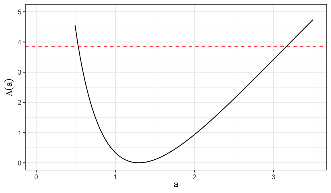
• 95% of $({\theta }_1/{\theta }_2)$ is the range of values of $a=({\theta }_1/{\theta }_2)$, such that $$\mathrm{\Lambda }(a)\le {\chi }_{(1),.95}^2=3.84$$ which is $$0.56<a<3.15\Rightarrow 0.56<({\theta }_1/{\theta }_2)<3.15$$

---

95% confidence interval of $({\theta }_1/{\theta }_2)$ for Type I censored sample

method	lower	upper
Normal approximation	0.54	3.114
LRT	0.56	3.150

Type II censored sample (CI for ${\theta }_1/{\theta }_2$)

• Lifetime distributions $T_i\sim \text{Exp}({\theta }_i)i=1,2$

• Type II censored sample for the group $i$, which has $r_i$ number of failures and $(n_i-r_i)$ subjects are censored at $t_{(i{r}_i)}$ $$t_{(i1)}<\cdots <t_{(i{r}_i)}$$

---

• Likelihood function $$\begin{array}{rl}L({\theta }_1,{\theta }_2)& =\prod _{i=1}^2(1/{\theta }_i{)}^{r_i}{e}^{-\sum _j{t}_{(ij)}/{\theta }_i}{e}^{-(n_i-r_i)t_{(i{r}_i)}/{\theta }_i}\\ & =\prod _{i=1}^2(1/{\theta }_i{)}^{r_i}{e}^{-(1/{\theta }_i)[\sum _j{t}_{(ij)}-(n_i-r_i)t_{(i{r}_i)}]}\\ & =\prod _{i=1}^2(1/{\theta }_i{)}^{r_i}{e}^{-T_i/{\theta }_i}\end{array}$$

---

• MLE $${\hat{\theta }}_i=\frac{T_i}{r_i}$$

• We have already shown that $$\frac{2T_i}{{\theta }_i}=\frac{2r_i{\hat{\theta }}_i}{{\theta }_i}\sim {\chi }_{(2r_i)}^2$$

• Then we can show $$\frac{(2r_1{\hat{\theta }}_1/{\theta }_1)/(2r_1)}{(2r_2{\hat{\theta }}_2/{\theta }_2)/(2r_2)}=\frac{{\hat{\theta }}_1{\theta }_2}{{\hat{\theta }}_2{\theta }_1}\sim F_{(2r_1,2r_2)}$$

---

• We can write $$P(F_{(2r_1,2r_2),\alpha /2}\le \frac{{\hat{\theta }}_1{\theta }_2}{{\hat{\theta }}_2{\theta }_1}\le F_{(2r_1,2r_2),1-\alpha /2})=1-\alpha$$

• $(1-\alpha )100\mathrm{\%}$ confidence interval for $({\theta }_1/{\theta }_2)$ $$\begin{array}{r}\frac{({\hat{\theta }}_1/{\hat{\theta }}_2)}{F_{(2r_1,2r_2),1-\alpha /2}}\le ({\theta }_1/{\theta }_2)\le \frac{({\hat{\theta }}_1/{\hat{\theta }}_2)}{F_{(2r_1,2r_2),\alpha /2}}\end{array}$$

4.2 Gamma distribution

• The pdf of two-parameter gamma distribution $$\begin{array}{r}f(t;\alpha ,k)=\frac{1}{\alpha \mathrm{\Gamma }k}(\frac{t}{\alpha }{)}^{k-1}\exp (-t/\alpha ),t>0\end{array}$$

  • Scale parameter $\alpha >0$ and shape parameter $k>0$

---

• Survivor function $$\begin{array}{rl}S(t;\alpha ,k)& ={\int }_t^{\mathrm{\infty }}f(u;\alpha ,k)du\\ & ={\int }_t^{\mathrm{\infty }}\frac{1}{\alpha \mathrm{\Gamma }k}(\frac{u}{\alpha }{)}^{k-1}\exp (-u/\alpha )du\\ & =1-I(k,t/\alpha )\end{array}$$

• Incomplete gamma function $$I(k,x)=\frac{1}{\mathrm{\Gamma }(k)}{\int }_0^x{u}^{k-1}{e}^{-u}du$$

Uncensored data

• Let $t_1,\dots ,t_n$ be a random sample from $\text{Gamma}(\alpha ,k)$, the log-likelihood function $$\begin{array}{rl}\ell (\alpha ,k)& =\sum _{i=1}^n\log f(t_i;\alpha ,k)\\ & =\sum _{i=1}^n\log [\frac{1}{\alpha \mathrm{\Gamma }k}(\frac{t_i}{\alpha }{)}^{k-1}\exp (-t_i/\alpha )]\\ & =-n\log \mathrm{\Gamma }k-nk\log \alpha +n(k-1)\log \tilde{t}-n\overline{t}/\alpha \end{array}$$

  • $\tilde{t}=(\prod _{i=1}^n{t}_i{)}^{1/n}$ and $\overline{t}=(1/n)\sum _i{t}_i$

---

$$\ell (\alpha ,k)=-n\log \mathrm{\Gamma }k-nk\log \alpha +n(k-1)\log \tilde{t}-n\overline{t}/\alpha$$

• Score functions $$\begin{array}{rl}{U}_1(\alpha ,k)& =\frac{\partial \ell (\alpha ,k)}{\partial \alpha }=\frac{-nk}{\alpha }+\frac{n\overline{t}}{{\alpha }^2}\\ U_2(\alpha ,k)& =\frac{\partial \ell (\alpha ,k)}{\partial k}=-n\psi (k)-n\log \alpha +n\log \tilde{t}\end{array}$$ where $\psi (k)={\mathrm{\Gamma }}^{\prime }(k)/\mathrm{\Gamma }(k)$ is the digamma function (see Appendix B of the Textbook)

---

• MLE $(\hat{\alpha },\hat{k})$ is a solution of the system of linear equations $$\begin{array}{rl}\frac{-n\hat{k}}{\hat{\alpha }}+\frac{n\overline{t}}{{\hat{\alpha }}^2}& =0\\ -n\psi (\hat{k})-n\log \hat{\alpha }+n\log \tilde{t}& =0\end{array}$$

  • Two equations and two unknowns

  • Equations are non-linear in terms of the variables

  • No closed form solutions

1. Substitution method

$$\begin{array}{}\text{(4.4)}& \frac{-n\hat{k}}{\hat{\alpha }}+\frac{n\overline{t}}{{\hat{\alpha }}^2}=0\Rightarrow \hat{\alpha }=\frac{\overline{t}}{\hat{k}}\end{array}$$

$$\begin{array}{}\text{(4.5)}& -n\psi (\hat{k})-n\log \hat{\alpha }+n\log \tilde{t}=0\Rightarrow \psi (\hat{k})-\log \hat{k}=\log (\tilde{t}/\overline{t})\end{array}$$

• Solve Equation 4.5 using a suitable optimization technique (e.g. graphical method, Newton-Raphson method, etc.) to obtain $\hat{k}$

• Then $\hat{\alpha }$ can be obtained from Equation 4.4

2. Newton-Raphson method

• Score functions $$\begin{array}{rl}{U}_1(\alpha ,k)& =\frac{\partial \ell (\alpha ,k)}{\partial \alpha }=\frac{-nk}{\alpha }+\frac{n\overline{t}}{{\alpha }^2}\\ U_2(\alpha ,k)& =\frac{\partial \ell (\alpha ,k)}{\partial k}=-n\psi (k)-n\log \alpha +n\log \tilde{t}\end{array}$$

---

• Elements of Hessian matrix $$\begin{array}{rl}{H}_{11}(\alpha ,k)& =\frac{{\partial }^2\ell (\alpha ,k)}{\partial {\alpha }^2}=\frac{nk}{{\alpha }^2}-\frac{2n\overline{t}}{{\alpha }^3}\\ H_{12}(\alpha ,k)& =\frac{{\partial }^2\ell (\alpha ,k)}{\partial \alpha \partial k}=\frac{-n}{\alpha }=I_{21}(\alpha ,k)\\ H_{22}(\alpha ,k)& =\frac{{\partial }^2\ell (\alpha ,k)}{\partial k^2}=-n{\psi }^{\prime }(k)\end{array}$$

---

• Score vector $$U(\alpha ,k)=\left[\begin{array}{c}{U}_1(\alpha ,k)\\ U_2(\alpha ,k)\end{array}\right]$$

• Hessian matrix $$H(\alpha ,k)=\left[\begin{array}{cc}{H}_{11}(\alpha ,k)& H_{12}(\alpha ,k)\\ H_{21}(\alpha ,k)& H_{22}(\alpha ,k)\end{array}\right]$$

• Score vector and information matrix are function of parameters and data

---

• Initial values ${\mathit{\theta }}^{(0)}=({\alpha }^{(0)},k^{(0)}{)}^{\prime }$ are chosen so that elements of score vector and hessian matrix are finite

• Updated estimate ${\mathit{\theta }}^{(1)}=({\alpha }^{(1)},k^{(1)}{)}^{\prime }$ is obtained as $$\begin{array}{}\text{(4.6)}& {\mathit{\theta }}^{(1)}={\mathit{\theta }}^{(0)}-[H({\mathit{\theta }}^{(0)}){]}^{-1}U({\mathit{\theta }}^{(0)})\end{array}$$

• The estimate ${\mathit{\theta }}^{(2)}$ can be obtained by using ${\mathit{\theta }}^{(1)}$ as input in Equation 4.6

• Repeating the procedure of evaluating the Equation 4.6 using the current estimate, the following sequence of estimates can be obtained $$\{{\mathit{\theta }}^{(j)},j=3,4,5,\dots \}$$

---

• A convergence criterion needs to be defined to obtain the MLE from the sequence of estimates $$\{{\mathit{\theta }}^{(j)},j=1,2,3,\dots \},$$

---

• Convergence criteria are defined on the basis of two successive values of the parameters estimates

• ${\mathit{\theta }}^{(j)}=(\hat{\alpha },\hat{k}{)}^{\prime }$ is considered as MLE if one of the following criteria is satisfied

  • $|{\mathit{\theta }}^{(j)}-{\mathit{\theta }}^{(j-1)}|\text{is very small}$

  • $|\ell ({\mathit{\theta }}^{(j)})-\ell ({\mathit{\theta }}^{(j-1)})|\text{is very small}$

  • $U({\mathit{\theta }}_j)\approx \mathbf{0}$

---

• Estimated variance-variance matrix of the MLE $(\hat{\alpha },\hat{k}{)}^{\prime }$ can be obtained from the inverse of the negative of the hessian matrix evaluated at the MLE $$\widehat{\text{Var}}\left(\begin{array}{c}\hat{\alpha }\\ \hat{k}\end{array}\right)=-[H(\hat{\alpha },\hat{k}){]}^{-1}$$

---

Newton-Raphson method: Pseudo code

1: theta0 <- `initial value of the parameter`
2: eps <- 1 
3: while (eps > 1e-5) {
4:   u0 <- U(theta0)
5:   h0 <- H(theta0)
6:   theat1 <- theta0 - inv(h0) * u0
7:   eps <- max(abs(theta1 - theta0))
8:   if (eps < 1e-5) break
9:   else theta0 <- theta1
10: }
11: return (list(theta0, h0))

---

• Statistical software have routines (such as optim() of R) that can optimize likelihood function to obtain MLE

  • Such routines require providing a “function” of likelihood function as an argument

  • Different optimization algorithms, such as Newton-Raphson, Mead-Nelder, simulated annealing, etc. are implemented in optimization routines

Statistical inference

• Asymptotic distributions of MLEs, i.e. $$\hat{\alpha }\sim \mathcal{N}(\alpha ,\text{var}(\hat{\alpha }))\text{and}\hat{k}\sim \mathcal{N}(k,\text{var}(\hat{k}))$$

• Since $\alpha >0$ and $k>0$, confidence intervals based on the sampling distribution of $\log \hat{\alpha }$ and $\log \hat{k}$ ensure non-negative lower limit of the confidence interval $$\log \hat{\alpha }\sim \mathcal{N}(\log \alpha ,\text{var}(\log \hat{\alpha }))\text{and}\log \hat{k}\sim \mathcal{N}(\log k,\text{var}(\log \hat{k}))$$

  • $\text{var}(\log \hat{\alpha })=(1/\hat{\alpha }{)}^2\text{var}(\hat{\alpha })$

---

• $(1-\alpha )100\mathrm{\%}$ confidence interval for $\log \alpha$

$$\log \hat{\alpha }\pm z_{1-\alpha /2}\text{SE}(\log \hat{\alpha })$$

• $(1-\alpha )100\mathrm{\%}$ confidence interval for $\alpha$

$$\hat{\alpha }\exp (\pm z_{1-\alpha /2}\text{SE}(\log \hat{\alpha }))$$

Example 4.2.1

Following are survival time of 20 male rates that were exposed to a high level of radiation

rtime <- c(152, 152, 115, 109, 137, 88, 94, 77, 160, 165, 125, 40, 128, 123, 136, 101, 62, 153, 83, 69)
rtime

 [1] 152 152 115 109 137  88  94  77 160 165 125  40 128 123 136 101  62 153  83
[20]  69

• Assume the lifetimes follow a gamma distribution with scale parameter $\alpha$ and shape parameter $k$

---

• From the data: $\overline{t}=113.45\text{and}\tilde{t}=107.07$

• Expressions of the score function $$\begin{array}{}\text{(4.7)}& \begin{array}{rl}\hat{\alpha }=(\overline{t}/\hat{k})& =113.45/\hat{k}\\ \psi (\hat{k})-\log \hat{k}-\log (\tilde{t}/\overline{t})& =0\\ \psi (\hat{k})-\log \hat{k}+0.058& =0\end{array}\end{array}$$

---

• R function uniroot() can be used to obtain the value of $\hat{k}$ by solving the Equation 4.7

kfun <- function(k0, time) {
  t_bar <- mean(time)
  tgbar <- exp(mean(log(time)))
  return(digamma(k0) - log(k0) - 
           log(tgbar / t_bar))
}
k_hat <- uniroot(kfun, lower = 3, 
                 upper = 10, 
                 time = rtime)

$$\hat{k}=8.799\Rightarrow \hat{\alpha }=12.893$$

k_hat

$root
[1] 8.799215

$f.root
[1] 8.181174e-10

$iter
[1] 7

$init.it
[1] NA

$estim.prec
[1] 6.103516e-05

Log-likelihood function of gamma distribution

• R function to calculate log-likelihood function of a gamma distribution for a given sample

gamma_loglk <- function(par, time) {
   sum(
     dgamma(time, scale = par[1], shape = par[2], log = T)
     )
}

• par is a vector with the parameter scale as the first element and shape as the second element

• time is the observed failure times

• gamma_loglk function can be evaluated for any given valid values of par and time

---

• For given values of parameters, say $({\alpha }_0=1,k_0=2.)$, the value of log-likelihood function can be obtained for the rat data

gamma_loglk(par = c(1, 2), time = rtime)

[1] -2175.531

• For another set of values $({\alpha }_0=100,k_0=80)$, the corresponding value of log-likelihood function

gamma_loglk(par = c(100, 80), time = rtime)

[1] -5392.711

optim() function

• R function optim() is a general purpose optimization routine

optim(par, fn,  gr = NULL, method = "Nelder-Mead",
      lower = -Inf, upper = Inf, 
      control = list(), hessian  = FALSE, ...
      )

• par $\to$ initial values for the parameters to be optimized

• fn $\to$ a function to be minimized

• gr $\to$ a function to return the gradient (score function)

• method $\to$ a method to be used, e.g. “Nelder-Mead”, “BFGS”, “CG”, “L-BFGS-B”, etc.

• lower and upper $\to$ lower and upper limit of the parameters to be optimized

• control $\to$ list of arguments (e.g. fnscale, etc.) for controlling the iterations

---

Initial values

• Initial values of the parameters can be selected from the exploratory plots of log-likelihood function

• The log-likelihood function must provide finite values with the initial values of the parameters

---

• As an example, assume the initial values ${\alpha }_0=12.9$ and $k_0=8.8$, and the corresponding value of log-likelihood function

gamma_loglk(par = c(12.9, 8.8), time = rtime)

[1] -100.48

• For another set of initial values, ${\alpha }_0=1.0$ and $k_0=1.0$

gamma_loglk(par = c(1.0, 1.0), time = rtime)

[1] -2269

---

• Since both sets of initial values can provide finite values of log-likelihood function, we can use either of these two as an initial value for optimizing the log-likelihood function using the R function optim()

Example 4.2.1 using optim()

• Fit of the gamma distribution to the rat data

gamma_fit <- optim(
    par = c(1, 1),  # initial values
    fn = gamma_loglk, # function name
    control = list(fnscale = -1), # for maximization
    hessian  = T, # will return hessian matrix
    time = rtime 
    )

---

• List of objects in gamma_fit

names(gamma_fit)

[1] "par"         "value"       "counts"      "convergence" "message"    
[6] "hessian"    

• Converged?

gamma_fit$convergence

[1] 0

---

• Estimate of scale and shape parameters

gamma_fit$par

[1] 12.896976  8.795312

• $\hat{\alpha }=12.897$ and $\hat{k}=8.795$

---

• Estimated variance-variance matrix

cvar <- solve(-gamma_fit$hessian)
cvar

          [,1]       [,2]
[1,]  16.88167 -10.871356
[2,] -10.87136   7.416138

• $\text{SE}(\hat{\alpha })=\sqrt{16.882}=4.109$

• $\text{SE}(\hat{k})=\sqrt{7.416}=2.723$

---

$95\mathrm{\%}$ CI for $\alpha$ and $k$

• Using the sampling distribution of $\hat{\alpha }$ and $\hat{k}$ $$\begin{array}{r}\hat{\alpha }\pm z_{1-\alpha /2}\text{SE}(\hat{\alpha })\Rightarrow 4.84\le \alpha \le 20.95\\ \hat{k}\pm z_{1-\alpha /2}\text{SE}(\hat{k})\Rightarrow 3.46\le \alpha \le 14.13\end{array}$$

• Using the sampling distribution of $\log \hat{\alpha }$ and $\log \hat{k}$ $$\begin{array}{r}\hat{\alpha }\exp (\pm z_{1-\alpha /2}\text{SE}(\log \hat{\alpha }))\Rightarrow 6.91\le \alpha \le 24.08\\ \hat{k}\exp (\pm z_{1-\alpha /2}\text{SE}(\hat{k}))\Rightarrow 4.79\le k\le 16.14\end{array}$$

---

Quantiles

• $p$th quantile $$\begin{array}{rl}S(t_p;\alpha ,k)=(1-p)& \Rightarrow \frac{1}{\mathrm{\Gamma }(k)}{\int }_{t_p/\alpha }^{\mathrm{\infty }}{u}^{k-1}{e}^{-u}du=(1-p)\\ & \Rightarrow (t_p/\alpha )=Q(p,k)\\ & \Rightarrow t_p=\alpha Q(p,k)\end{array}$$

  • $Q(p,k)$ is the $p$th quantile function of one-parameter gamma distribution [R function qgamma(p, scale=1, shape)]

• Estimate of the median for the rat data is ${\hat{t}}_{.5}=\hat{\alpha }Q(.5,\hat{k})$

12.893951 * qgamma(.5, scale = 1, shape = 8.799089)     

[1] 109.1872

qgamma(.5, scale = 12.893951, shape = 8.799089)

[1] 109.1872

Likelihood ratio statistic

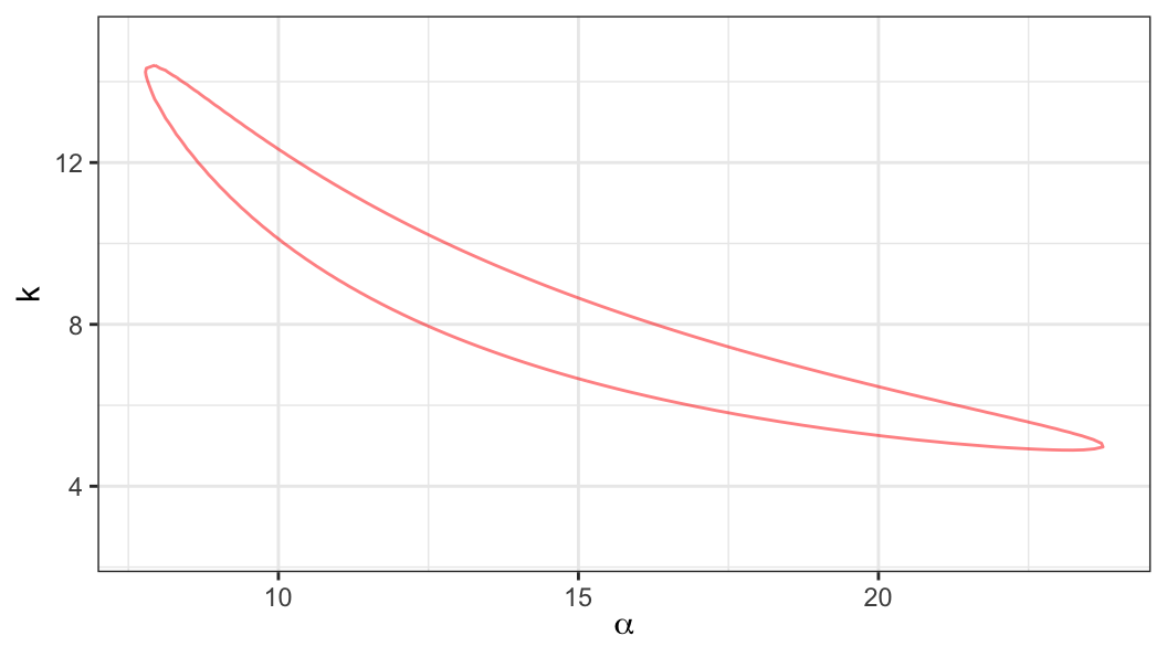
• Likelihood ratio statistic $$\mathrm{\Lambda }(\alpha ,k)=2\ell (\hat{\alpha },\hat{k})-2\ell (\alpha ,k)$$

• Approximate $(1-p)100\mathrm{\%}$ confidence region for $(\alpha ,k{)}^{\prime }$ can be obtained from the set of points $(\alpha ,k)$ satisfying $$\mathrm{\Lambda }(\alpha ,k)\le {\chi }_{(2),1-p}^2$$

---

95% confidence region of $(\alpha ,k)$ for rat survival data

LRT statistic based CI for $k$

• Consider the following null hypothesis $$H_0:k=k_0$$

• MLEs (unrestricted and under restriction) $$\begin{array}{r}(\hat{\alpha },\hat{k})={argmax}_{(\alpha ,k)\in \mathrm{\Theta }}\ell (\alpha ,k)\text{under }{H}_1\\ \tilde{\alpha }(k_0)={argmax}_{\alpha \in {\mathrm{\Theta }}_{\alpha }}\ell (\alpha ,k_0)\text{under }{H}_0\end{array}$$

---

• Likelihood ratio statistic $$\begin{array}{r}{\mathrm{\Lambda }}_k(k_0)=2\ell (\hat{\alpha },\hat{k})-2\ell (\tilde{\alpha }(k_0),k_0)\end{array}$$

  • Under $H_0:k=k_0$, ${\mathrm{\Lambda }}_k(k_0)$ approximately follows a ${\chi }_{(1)}^2$ distribution

• An approximate two-sided $(1-p)100\mathrm{\%}$ confidence interval for $k$ can be obtained from a set of values of $k_0$ satisfying $$\begin{array}{r}{\mathrm{\Lambda }}_k(k_0)\le {\chi }_{(1),1-p}^2\end{array}$$

---

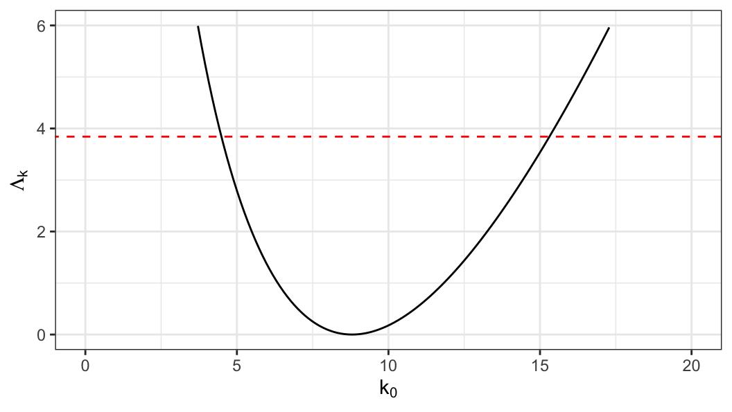
$$\text{95\% CI}:4.54\le k\le 15.28$$

LRT statistic based CI for $\alpha$

• Consider the following null hypothesis $$H_0:\alpha ={\alpha }_0$$

• MLEs (unrestricted and under restriction) $$\begin{array}{r}(\hat{\alpha },\hat{k})={argmax}_{(\alpha ,k)\in \mathrm{\Theta }}\ell (\alpha ,k)\text{under }{H}_1\\ \tilde{k}({\alpha }_0)={argmax}_{k\in {\mathrm{\Theta }}_k}\ell ({\alpha }_0,k)\text{under }{H}_0\end{array}$$

---

• Likelihood ratio statistic $$\begin{array}{r}{\mathrm{\Lambda }}_{\alpha }({\alpha }_0)=2\ell (\hat{\alpha },\hat{k})-2\ell ({\alpha }_0,\tilde{k}({\alpha }_0))\end{array}$$

  • Under $H_0:\alpha ={\alpha }_0$, ${\mathrm{\Lambda }}_{\alpha }({\alpha }_0)$ approximately follows a ${\chi }_{(1)}^2$ distribution

• An approximate two-sided $(1-p)100\mathrm{\%}$ confidence interval for $\alpha$ can be obtained from a set of values of ${\alpha }_0$ satisfying $$\begin{array}{r}{\mathrm{\Lambda }}_{\alpha }({\alpha }_0)\le {\chi }_{(1),1-p}^2\end{array}$$

---

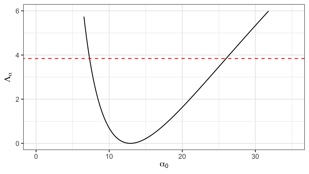
$$\text{95\% CI}:7.37\le \alpha \le 25.9$$

---

Summary of $95\mathrm{\%}$ CI

• For $\alpha$ $$\begin{array}{rl}\text{no-transformation}:& 4.84\le \alpha \le 20.95\\ \text{log-transformation}:& 6.91\le \alpha \le 24.08\\ \text{LRT}:& 7.37\le \alpha \le 25.9\end{array}$$

• For $k$ $$\begin{array}{rl}\text{no-transformation}:& 3.46\le k\le 14.13\\ \text{log-transformation}:& 4.79\le k\le 16.14\\ \text{LRT}:& 4.54\le k\le 15.28\end{array}$$

Censored

Data $\{(t_i,{\delta }_i),i=1,\dots ,n\}$ and the corresponding log-likelihood function $$\begin{array}{rl}\ell (\alpha ,k)& =\log \prod _{i=1}^n[\frac{1}{\alpha \mathrm{\Gamma }(k)}(\frac{t_i}{\alpha }{)}^{k-1}{e}^{-t_i/\alpha }{]}^{{\delta }_i}[1-I(k,t_i/\alpha ){]}^{1-{\delta }_i}\\ & =-k\log \alpha -r\log \mathrm{\Gamma }(k)+(k-1)\sum _i{\delta }_i\log t_i\\ & -\sum _i{\delta }_i{t}_i/\alpha +\sum _i(1-{\delta }_i)\log [1-I(k,t_i/\alpha )]\end{array}$$

---

• No closed form solutions are available for MLEs $\hat{\alpha }$ and $\hat{k}$

• Algebraic expressions of score function and information matrix for the log-likelihood function $\text{(???)}$ are very complicated

• Score functions and information matrix can be evaluated numerically

• Optimization routines available in statistical software can be used to obtain MLEs $\hat{\alpha }$ and $\hat{k}$, and the corresponding SEs

  • Different optimization algorithms such as Newton-Raphson, Nelder-Mead, etc. are available in such routines

---

• As an example, we are going to use the same rat data that we have used for the analysis of complete data

• For the rat data, assume a time $\ge 150$ weeks is considered as censored, there are 5 censored observations

  • An R object rtimec is created, which has two columns time and status

rtimec |> t()

       [,1] [,2] [,3] [,4] [,5] [,6] [,7] [,8] [,9] [,10] [,11] [,12] [,13]
time    152  152  115  109  137   88   94   77  160   165   125    40   128
status    0    0    1    1    1    1    1    1    0     0     1     1     1
       [,14] [,15] [,16] [,17] [,18] [,19] [,20]
time     123   136   101    62   153    83    69
status     1     1     1     1     0     1     1

---

gamma log-likelihood function for censored sample

gamma_loglk <- function(par, time, status = NULL) {
  #
  if (is.null(status)) status <- rep(1, length(time))
  #
  llk_f <- sum(status * dgamma(time, scale = par[1], 
                  shape = par[2], log = T))
  #
  llk_c <- sum((1 - status) * pgamma(time, scale = par[1], 
                     shape = par[2], lower.tail = F, 
                     log.p = T))
  return(llk_f + llk_c)
}

Censored sample

• R codes to obtain MLE of parameters of a gamma distribution from a censored sample

gamma_out_c <- optim(
  par = c(1, 1), fn = gamma_loglk, 
  control = list(fnscale = -1), hessian  = T, 
  time = rtimec$time, status = rtimec$status
)

---

• Maximum likelihood estimators [gamma_out_c$par] $$\hat{\alpha }=21.3\text{and}\hat{k}=5.79$$

• Standard errors [solve(-gamma_out_c$hessian)] $$se(\hat{\alpha })=8.61\text{and}se(\hat{k})=2.14$$

---

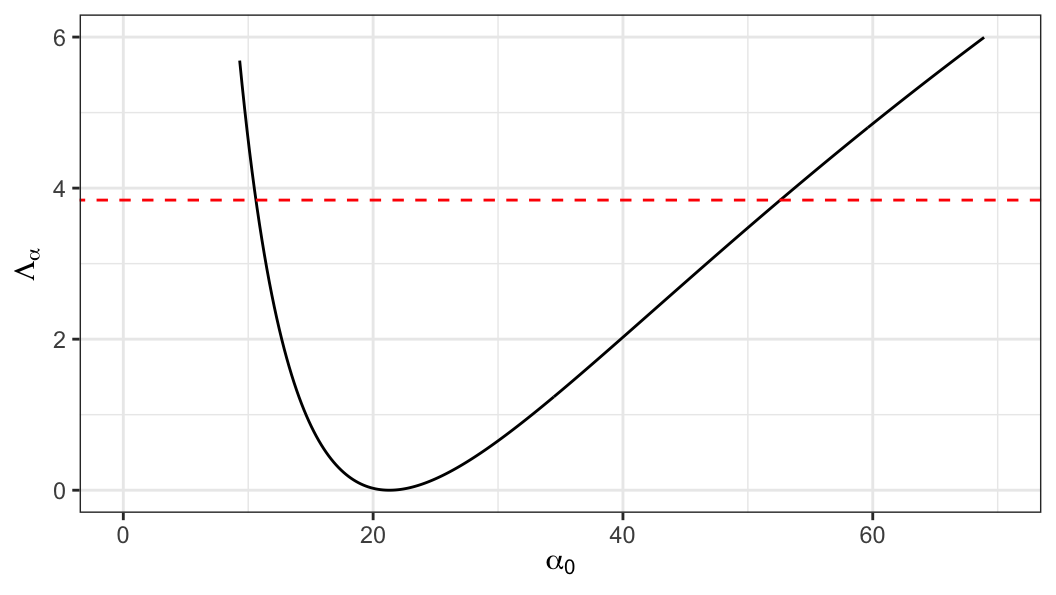
$$\text{95\% CI}:10.7\le \alpha \le 52.48$$

---

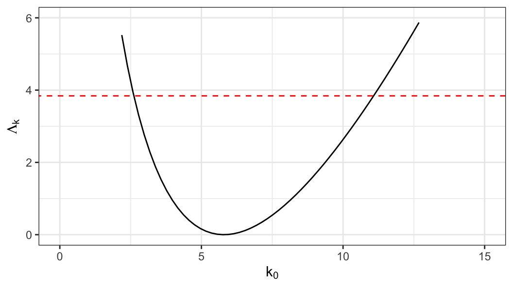
$$\text{95\% CI}:2.78\le k\le 10.9$$

---

• $95\mathrm{\%}$ CI for $\alpha$ $$\begin{array}{rl}\text{no-transformation}:& 4.44\le \alpha \le 38.17\\ \text{log-transformation}:& 9.65\le \alpha \le 47.02\\ \text{LRT}:& 10.7\le \alpha \le 52.48\end{array}$$

• $95\mathrm{\%}$ CI for $k$ $$\begin{array}{rl}\text{no-transformation}:& 3.46\le k\le 14.13\\ \text{log-transformation}:& 4.79\le k\le 16.14\\ \text{LRT}:& 2.78\le k\le 10.9\end{array}$$

---

• Estimate of median $${\hat{t}}_{.5}=\hat{\alpha }Q(.5,\hat{k})=116.4\text{weeks}$$

---

Acknowledgements

This lecture is adapted from materials created by Mahbub Latif

References

Sprott, David Arthur. 1980. “Maximum Likelihood in Small Samples: Estimation in the Presence of Nuisance Parameters.” Biometrika 67 (3): 515–23.