Linear Regression Review

(AST405) Lifetime data analysis

Authors

Affiliation

0 Linear Regression Models

0.1 Multiple Linear Regression Models

Multiple Linear Regression Models

• Let $\{(y_i,x_{i1},\dots ,x_{ip}),i=1,\dots ,n\}$ be the data obtained from the $i^{th}$ subject

  • $y_i\to$ response

  • $x_{ij}\to$ $jth$ independent variable

---

• A multiple linear regression model $$y_i={\beta }_0+{\beta }_1{x}_{i1}+\cdots +{\beta }_p{x}_{ip}+{ϵ}_{ij}$$

• In matrix notation $$\mathbf{y}={\mathbf{x}}^{\prime }\mathit{\beta }+\mathit{ϵ}$$

  • $\mathbf{y}=(y_1,\dots ,y_n{)}^{\prime }$

  • $\mathbf{x}\to$ $n\times (p+1)$ matrix with first column is a vector of one’s

  • $\mathit{\beta }=({\beta }_0,{\beta }_1,\dots ,{\beta }_p{)}^{\prime }$

  • ${ϵ}_{ij}\to$ error term

---

• General assumptions

  • $ϵ$’s are independent

  • $E({ϵ}_{ij})=0$

  • $V({ϵ}_{ij})={\sigma }^2$

  • ${ϵ}_{ij}\sim N(0,{\sigma }^2)$

---

• The fitted model $${\hat{y}}_i={\hat{\beta }}_0+{\hat{\beta }}_1{x}_{i1}+\cdots +{\hat{\beta }}_p{x}_{ip}$$

  • Ordinary least squares or maximum likelihood estimators $$\hat{\mathit{\beta }}=({\mathbf{x}}^{\prime }\mathbf{x}{)}^{-1}{\mathbf{x}}^{\prime }\mathbf{y}$$

  • Asymptotically $\hat{\mathit{\beta }}$ follows a normal distribution with mean vector $\mathit{\beta }$ and variance-covariance matrix $({\mathbf{x}}^{\prime }\mathbf{x}{)}^{-1}{\sigma }^2$

---

• Residuals $$\widehat{\mathit{ϵ}}=\mathbf{y}-\hat{\mathbf{y}}$$

  • Estimate of error variance $${\hat{\sigma }}^2=\frac{{\mathit{ϵ}}^{\prime }\mathit{ϵ}}{n-p-1}$$

  • Residuals are used for model diagnostics

---

• Statistical inference regarding multiple linear regression models are based on t-test, F-test, and chi-square test

$$\begin{array}{rl}{H}_{01}& :{\beta }_j=0(j=1,\dots ,p)\\ H_{02}& :{\beta }_1=\cdots ={\beta }_p=0\\ H_{03}& :{\beta }_1=\cdots ={\beta }_q=0(q<p)\\ H_{04}& :{\beta }_1=\cdots ={\beta }_q(q<p)\end{array}$$

0.2 An example with data on inheritance of height

Inheritance of height

• During 1893–1898 in the UK, K. Pearson (a famous statistician) organized the collection of heights of 1375 mothers aged 65 or less and one of their adult daughters aged 18 or more (Pearson and Lee 1903)

  • Mother height $(x)$ $\to$ predictor

  • Daughter height $(y)$ $\to$ response

Does taller mother tend to have taller daughter?

• Assumed model “Daughter height on mother height” $$y_i={\beta }_0+{\beta }_1{x}_i+{ϵ}_i$$

Inheritance of height

• The data heights

library(alr4)
data("Heights")

• Transform Heights from data.frame() to tibble()

heights <- as_tibble(Heights)

Scatterplot of mother height and daughter height

ggplot(heights) + 
  geom_point(aes(mheight, dheight), size = .75) +
  theme_bw()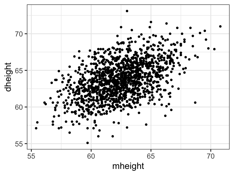

---

0.3 Model fit

lm()

• lm() is the most popular R function to fit linear model (with continuous response)

  • A typical syntax of lm() function lm(formula, data), which returns a list

• For example, codes for fitting the model “Daughter height on mother height”

mod_h <- lm(formula = dheight ~ mheight,
            data = heights)

---

• Elements of lm() output object contain useful objects related to the corresponding fit of linear model

names(mod_h)

 [1] "coefficients"  "residuals"     "effects"       "rank"         
 [5] "fitted.values" "assign"        "qr"            "df.residual"  
 [9] "xlevels"       "call"          "terms"         "model"        

mod_h$coefficients

(Intercept)     mheight 
  29.917437    0.541747 

---

• Elements of lm() output object contain useful objects related to the corresponding fit of linear model

names(summary(mod_h))

 [1] "call"          "terms"         "residuals"     "coefficients" 
 [5] "aliased"       "sigma"         "df"            "r.squared"    
 [9] "adj.r.squared" "fstatistic"    "cov.unscaled" 

summary(mod_h)$coefficients

             Estimate Std. Error  t value     Pr(>|t|)
(Intercept) 29.917437 1.62246940 18.43945 5.211879e-68
mheight      0.541747 0.02596069 20.86797 3.216915e-84

---

• Output of lm() object can also be used as an argument of some useful functions, such as

  • coefficients() returns the estimates of regression parameters

  • residuals() returns associated residuals (there are different types of residuals, use type argument to specify this)

  • fitted() returns fitted values corresponding to the predictor values of the data

  • anova() returns ANOVA table

  • summary() returns objects related to linear model fits, some of them are not included in the lm() object

  • confint() returns confidence intervals of the regression parameters

0.4 broom package

broom

• Most of the built-in R objects related to model fits (e.g. lm(), t.test(), etc.) require tidy data as input, but its outputs are messy (not tidy), which cannot be used as input for the methods of tidyverse

  • e.g. lm() returns a list, not a data frame

• broom package has functions that transform messy data into tidy data, which are used as inputs of different tidyverse functions, such as ggplot(), kable(), etc.

---

• broom has three functions that takes model fit object as an argument and returns a tibble (tidy data)

  • glance() returns a signle row summary of the model fit, which contains estimates of coefficient of determination, error variance, etc.

  • tidy() returns different values corresponding to each parameter, such as estimates, t-stat, p-value, etc.

  • augment() returns fitted information corresponding to each observations, e.g. residuals, fitted values, SE of fitted values, etc.

glance()

Single row summary of the model fit

glance(mod_h)

# A tibble: 1 × 12
  r.squared adj.r.squared sigma statistic  p.value    df logLik   AIC   BIC
      <dbl>         <dbl> <dbl>     <dbl>    <dbl> <dbl>  <dbl> <dbl> <dbl>
1     0.241         0.240  2.27      435. 3.22e-84     1 -3075. 6156. 6172.
# ℹ 3 more variables: deviance <dbl>, df.residual <int>, nobs <int>

tidy()

Summary of the parameter estimates

tidy(mod_h)

# A tibble: 2 × 5
  term        estimate std.error statistic  p.value
  <chr>          <dbl>     <dbl>     <dbl>    <dbl>
1 (Intercept)   29.9      1.62        18.4 5.21e-68
2 mheight        0.542    0.0260      20.9 3.22e-84

augment()

Observation-wise values of model fit

augment(mod_h) %>%
  slice(1:6)

# A tibble: 6 × 8
  dheight mheight .fitted .resid     .hat .sigma .cooksd .std.resid
    <dbl>   <dbl>   <dbl>  <dbl>    <dbl>  <dbl>   <dbl>      <dbl>
1    55.1    59.7    62.3  -7.16 0.00172    2.26 0.00862     -3.16 
2    56.5    58.2    61.4  -4.95 0.00310    2.26 0.00743     -2.19 
3    56      60.6    62.7  -6.75 0.00118    2.26 0.00523     -2.98 
4    56.8    60.7    62.8  -6.00 0.00113    2.26 0.00397     -2.65 
5    56      61.8    63.4  -7.40 0.000783   2.26 0.00418     -3.27 
6    57.9    55.5    60.0  -2.08 0.00707    2.27 0.00303     -0.923

0.5 Model diagnostics

Model diagnostics

• Residual vs fitted (Independence of errors, Constant variance)

• Residual vs predictor (Linearity, Zero mean)

• Q-Q normal plot of residuals (Normality of error)

Residual plots

Scatterplot of fitted values and residuals

ggplot(augment(mod_h)) +
  geom_point(aes(.fitted, .resid), size = .75) +
  labs(x = "fitted", y = "residuals") + 
  theme_minimal()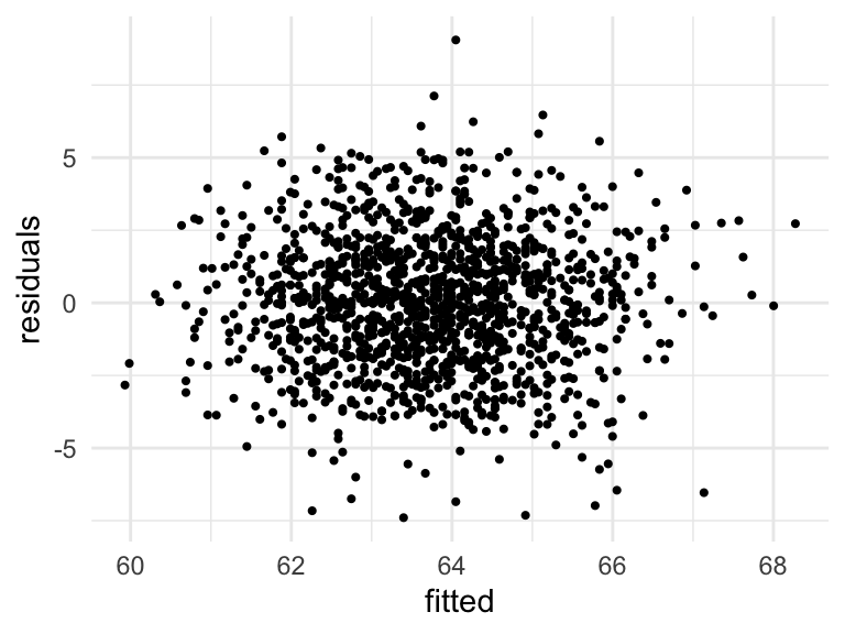

---

---

Scatterplot of predictor and residuals

ggplot(augment(mod_h)) +
  geom_point(aes(mheight, .resid), size = .75) +
  labs(x = "Mother Ht", y = "residuals") + 
  theme_minimal()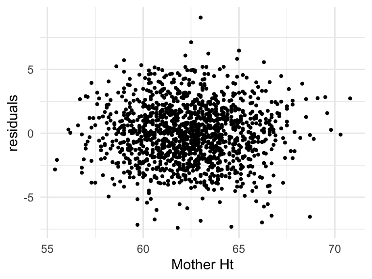

---

Q-Q normal plot

Using base R functions

qqnorm(residuals(mod_h))
qqline(residuals(mod_h))

---

---

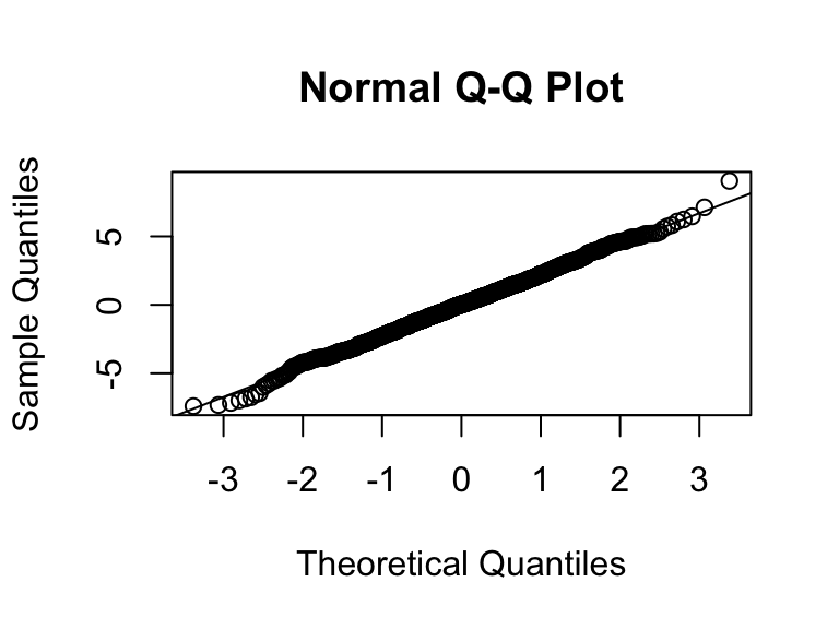
• For Q-Q plot, ggplot2 functions stat_qq() and stat_qq_line() can be used

ggplot(augment(mod_h), aes(sample = .resid)) +
  stat_qq() +
  stat_qq_line() +
  theme_minimal()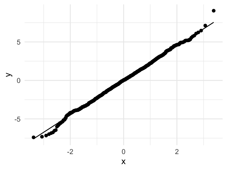

---

Summary

• lm() function is used to fit the models

• Functions of broom package can be used to obtain tidy data from the output of lm() function, which is usually messy

• Output of functions of broom package can be used as arguments of ggplot and other tidyverse functions

Exercise

• Using the FEV data (Download the FEV data), fit the following models and perform the model diagnostics

  1. fev on Age

  2. fev on Age and Hgt

0.6 Regression models with categorical predictors

Regression models with categorical predictors

• In general, for a predictor with two levels, define a dummy or binary variable that takes the values 1 and 0 corresponding to the two levels of the original variable

  • For example, if the variable $X$ has the levels “male” and “female”, we can define a dummy variable $D$ such that $$D=\{\begin{array}{ll}1& \text{if }X=\text{male}\\ 0& \text{if }X=\text{female}\end{array}$$

  • The level “female” is considered as the “reference” category in this case

  • Dummy variable can also be defined with “male” as the reference category

---

• The model “$Y$ on $X$” can be expressed in terms of “$D$” as $$E(Y|D)={\beta }_0+{\beta }_{1}D$$

  • ${\beta }_0=E(Y|D=0)$

  • ${\beta }_1=E(Y|D=1)-E(Y|D=0)$

• Interpretations of regression parameters depend on the reference category considered

---

• For a categorical variable with more that two categories, more than one dummy variables needed to be defined

• Let $X$ be a categorical variable with three categories, say “poor”, “middle”, and “rich”

  • To consider $X$ as a predictor, two dummy variables need to be defined $$\begin{array}{rl}{D}_1=\{\begin{array}{ll}1& \text{if }X=\text{poor}\\ 0& \text{otherwise}\end{array}& D_2=\{\begin{array}{ll}1& \text{if }X=\text{middle}\\ 0& \text{otherwise}\end{array}\end{array}$$

  • In this case, the category “rich” is considered as the reference category and dummy variables can be defined with other category as the reference

---

• The regression model “$Y$ on $X$”, where $X$ has three categories can be defined as $$E(Y|D_1,D_2)={\beta }_0+{\beta }_1{D}_1+{\beta }_2{D}_2$$

  • ${\beta }_0=E(Y|D_1=0,D_2=0)$

  • ${\beta }_1=E(Y|D_1=1,D_2=0)-E(Y|D_1=0,D_2=0)$

  • ${\beta }_2=E(Y|D_1=0,D_2=1)-E(Y|D_1=0,D_2=0)$

0.7 Interaction

Regression models with one categorical and one continuous predictors

• Consider a regression model “$Y$ on $X_1$ and $X_2$”, where $X_1$ has two levels (“male” and “female”) and $X_2$ is continuous (say age in years)

• Define a dummay variable for $X_1$

  • $D_{1M}=I(X_1=\text{Male})$

---

Consider the models $$\begin{array}{rl}(1)E(Y|D_{1M},X_2)& ={\beta }_0+{\beta }_1{D}_{1M}+{\beta }_2{X}_2\\ (2)E(Y|D_{1M},X_2)& ={\beta }_0+{\beta }_1{D}_{1M}+{\beta }_2{X}_2+\theta D_{1M}{X}_2\end{array}$$

• How would you interpret the parameters in model (1)?
• How would you interpret $\theta$ in model (2)?

---

$$\begin{array}{rl}(2)E(Y|D_{1M},X_2)& ={\beta }_0+{\beta }_1{D}_{1M}+{\beta }_2{X}_2+\theta D_{1M}{X}_2\\ & =\{\begin{array}{ll}{\beta }_0+{\beta }_2{X}_2& \text{for female}\\ ({\beta }_0+{\beta }_1+({\beta }_2+\theta )X_2& \text{for male}\end{array}\end{array}$$

• ${\beta }_0\to$ mean response of female of age 0

• ${\beta }_1\to$ difference of mean response between male and female when both of them at age of 0

• ${\beta }_2\to$ change of mean response for 1 year change in age for female

• $\theta \to$ difference in the change of the mean response between males and females when their age changes by 1 year

  • it represents how the effect of age differs between males and females

---

Regression model with two categorical variables

• Consider a regression model “$Y$ on $X_1$ and $X_2$”, where $X_1$ has two levels (“male” and “female”) and $X_2$ has three levels (“poor”, “middle”, and “rich”)

• Define the dummy variables for the categorical variables $X_1$ and $X_2$

  • For $X_1$, $D_{1M}=I(X_1=\text{male})$

  • For $X_2$, $D_{21}=I(X_2=\text{poor})$ and $D_{22}=I(X_2=\text{middle})$

---

Model 1

$$E(Y|D_{1M},D_{21},D_{22})={\beta }_0+{\beta }_1{D}_{1M}+{\beta }_{21}{D}_{21}+{\beta }_{22}{D}_{22}$$

• ${\beta }_0\to$ mean response of rich female individuals

• ${\beta }_1\to$ mean difference between male and female when $X_2$ is fixed

• ${\beta }_{21}\to$ mean difference between poor and rich when $X_1$ is fixed

• ${\beta }_{22}\to$ mean difference between middle and rich when $X_1$ is fixed

---

Model 2

• The “Model 2” contains both main effects and interactions $$\begin{array}{rl}E(Y|D_{1M},D_{21},D_{22})& ={\beta }_0+{\beta }_1{D}_{1M}+{\beta }_{21}{D}_{21}+{\beta }_{22}{D}_{22}\\ & +{\theta }_1{D}_{1M}{D}_{21}+{\theta }_2{D}_{1M}{D}_{22}\end{array}$$

  • ${\beta }_0\to$ mean response of rich female individuals

  • Interpretations of other parameters are complicated!!

---

• The following table of expected response would help us to define parameters of “Model 2”

$$\overline{)\begin{array}{llll}\text{ gender }& \text{ Poor }& \text{ Middle }& \text{ Rich }\\ \text{ Male }& {\beta }_0+{\beta }_1+{\beta }_{21}+{\theta }_1& {\beta }_0+{\beta }_1+{\beta }_{22}+{\theta }_2& {\beta }_0+{\beta }_1\\ \text{ Female }& {\beta }_0+{\beta }_{21}& {\beta }_0+{\beta }_{22}& {\beta }_0\end{array}}$$

• Interpret $\theta$’s

---

• Difference of mean response between male and female among the “rich” $$E(Y|\text{Male},\text{Rich})-E(Y|\text{Female},\text{Rich})={\beta }_1$$

• Difference of mean response between male and female among the “middle” $$E(Y|\text{Male},\text{Middle})-E(Y|\text{Female},\text{Middle})={\beta }_1+{\theta }_1$$

---

• Difference in differences (DID) $$\begin{array}{rl}\{E(Y|\text{Male},\text{Middlw})-E(Y|\text{Female},\text{Middle})\}& \\ -\{E(Y|\text{Male},\text{Rich})-E(Y|\text{Female},\text{Rich})\}& ={\theta }_1\end{array}$$

• Interaction term ${\theta }_1$ measures whether the effect of “gender” is the same at the levels “Rich” and “Middle”

• Similarly, the interaction term ${\theta }_2$ measures whether the effect of “gender” is the same at the levels “Rich” and “Poor”

---

• In the presence of significant interactions, the main effects have no interesting interpretations

• Interaction terms should not be in the model if both the corresponding main effects are not significant

• Insignificant interaction terms should not be in the model

Acknowledgements

This lecture is adapted from materials created by Mahbub Latif

References

Pearson, Karl, and Alice Lee. 1903. “On the Laws of Inheritance in Man: I. Inheritance of Physical Characters.” Biometrika 2 (4): 357–462.