Chapter 6

(AST405) Lifetime data analysis

6 Parametric Regression Models

6.1 Log-location-scale (Accelerated Failure Time) Regression Models

Linear regression model

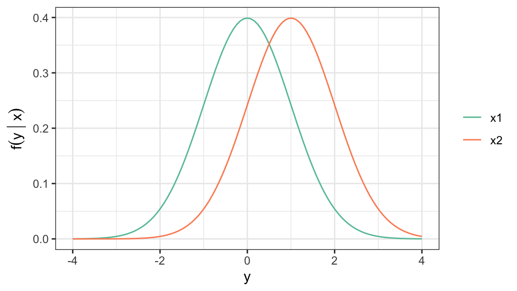
• Distributional assumption for the response \[ (Y\,\vert\, x)=Y(x) \sim \mathcal{N}\big(\mu(x), \sigma^2\big) \]
• Regression model for the parameters \[\begin{aligned} \mu(x) & = \beta_0 + \beta_1x_1 + \cdots + \beta_px_p = \mathbf{x}'\boldsymbol{\beta}\\[.25em] \operatorname{var} (Y\,\vert\, x) & = \sigma^2 \end{aligned}\]

---

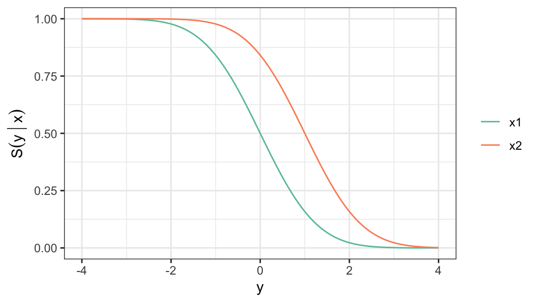
• Instead of the parameters, linear regression model can be defined in terms of other functions, such as survivor function \[ \begin{aligned} S_Y(y) & = Pr(Y > y) \notag \\[.2em] & = 1 -\Phi\bigg(\frac{y - \mu(x)}{\sigma}\bigg) \end{aligned} \tag{6.1}\]

Regression models for lifetimes

• Similar to continuous and binary responses, regression analysis of lifetimes involves specifications for the distribution of a lifetime \((T)\) given a vector of \(p\)-dimensional (say) covariate \(\mathbf{x}\) \[ (T\,\vert\, \mathbf{x}) = T(\mathbf{x}) \]

---

• For parametric regression models for lifetimes \(T\), parameters (e.g. scale and shape parameters) need to be defined as a function of measured covariates (linear predictors)

• It requires selecting a link function (e.g. identity, log, logit, etc.) for relating model parameters with linear predictors

• Similar to linear and logistic regression models, maximum likelihood method of estimation is used to estimate parameters of the model

Log-location-scale AFT model

• For a lifetime that follows a distribution of the log-location-scale family of distributions, the survivor function of lifetime \(T\) for a given covariate vector \(\mathbf{x}\) is defined as \[ S(t\,\vert\, \mathbf{x}) = S_0^{\star}\Big([t/\alpha(\mathbf{x})]^{\delta}\Big) \tag{6.2}\]

  • Scale parameter \(\alpha(\mathbf{x})\) is defined as a function of covariate vector \(\mathbf{x}\)

  • Shape parameter \(\delta\) does not depend on \(\mathbf{x}\)

  • Survivor function of the corresponding standardized distribution \(S_0^{\star}(x)=S_0(\log x)\) is defined earlier

---

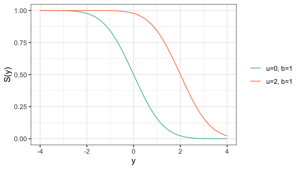
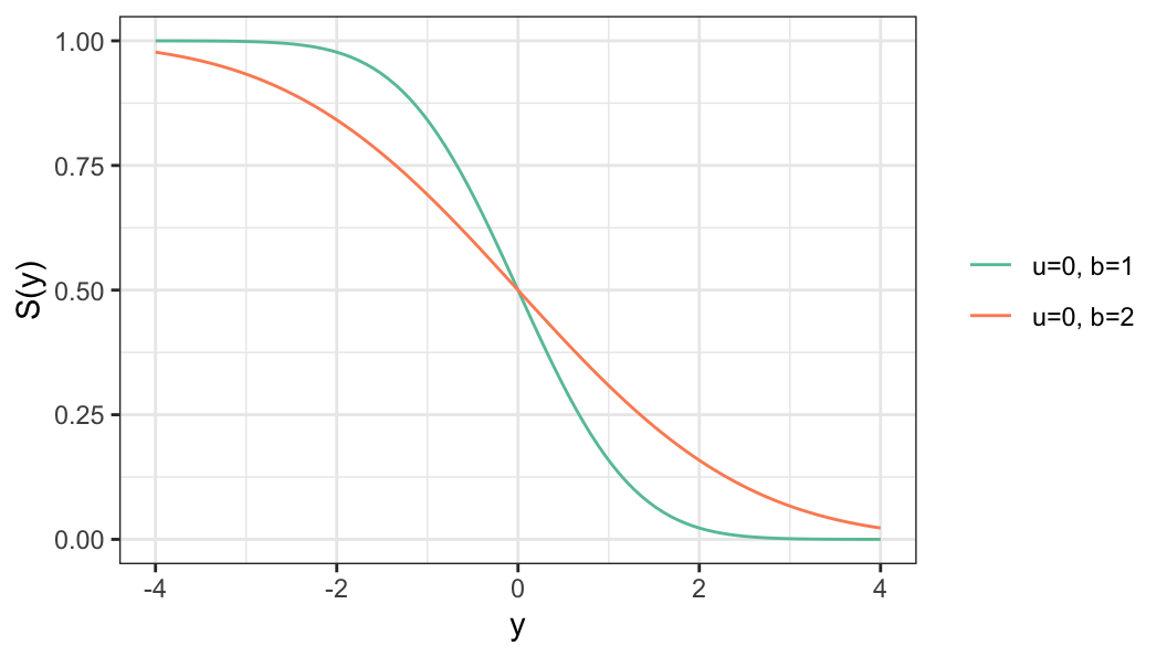
• For a log-lifetime that follows a distribution of the location-scale family of distribution, the survivor function of log-lifetime \(Y\) for a given covariate vector \(\mathbf{x}\) is defined as \[ S(y\,\vert\, \mathbf{x}) = S_0\bigg(\frac{y-u(\mathbf{x})}{b}\bigg) \tag{6.3}\]

  • Location parameter \(u(\mathbf{x})\) is defined as a function covariate vector \(\mathbf{x}\)

  • Scale parameter \(b\) does not depend on \(\mathbf{x}\)

• The model (Equation 6.3) for log-lifetime is similar to the linear regression model (Equation 6.1) with \[\mu(\mathbf{x})=u(\mathbf{x}), \sigma =b, \;\text{and}\; \Phi(x) = 1 - S_0(x)\]

---

• The model for lifetime (Equation 6.2) or log-lifetime (Equation 6.3) is known as accelerated failure time (AFT) model \[ \begin{aligned} S(t\,\vert\, \mathbf{x}) & = S_0^{\star}\Big([t/\alpha(\mathbf{x})]^{\delta}\Big) \\[.25em] S(y\,\vert\, \mathbf{x}) &= S_0\bigg(\frac{y-u(\mathbf{x})}{b}\bigg) \end{aligned} \]

• Models for the parameters \(\alpha(\mathbf{x})\) and \(u(\mathbf{x})\) are defined so that associated parametric restrictions are satisfied, \(\alpha(\mathbf{x})>0\) and \(-\infty <u(\mathbf{x})<\infty\), e.g. \[ \begin{aligned} u(\mathbf{x}) &=\beta_0 + \beta_1x_1 + \cdots + \beta_px_p = \mathbf{x}'\boldsymbol{\beta} \\[.25em] \alpha(\mathbf{x}) &= \exp \big(\mathbf{x}'\boldsymbol{\beta}\big) \end{aligned} \]

---

• AFT model can also be expressed as \[ \frac{Y-u(\mathbf{x})}{b} = Z \quad\Rightarrow\quad{\color{purple}Y = u(\mathbf{x}) + bZ} \tag{6.4}\]

  • \(Z\sim S_0(z)\), i.e. \(Z\) follows a standardized log-location-scale distribution, e.g. standard normal or extreme-value distributions with location 0 and scale 1, etc.

• Linear regression model (Equation 6.1) can also be expressed as Equation 6.4: \[ Y = \mu(\mathbf{x}) + \sigma Z, \quad Z\sim \mathcal{N}(0, 1) \]

---

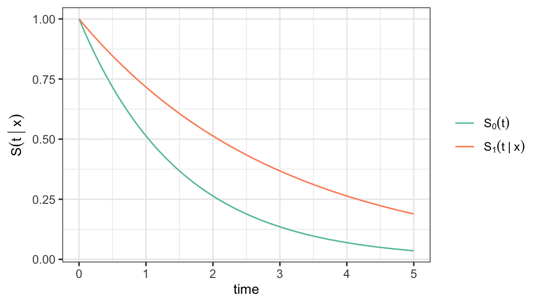
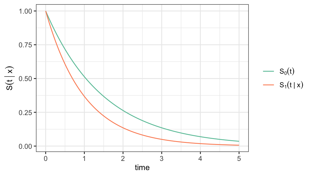
• In AFT model defined in terms of the distribution of lifetime \(T\), covariates alter the time scale

  • If \(\alpha(\mathbf{x})= \exp \big(\mathbf{x}'\boldsymbol{\beta}\big) >1\), the effect of covariate vector is to increase time (decelerate time)

  • If \(\alpha(\mathbf{x})= \exp \big(\mathbf{x}'\boldsymbol{\beta}\big)<1\), the effect of covariate vector is to shorten time (accelerate time)

---

• The accelerated failure time model is a general model for survival data, in which explanatory variables measured on an individual are assumed to act multiplicatively on the time-scale

• Log-location-scale AFT models are a special case of AFT models where the log of survival time follows a location-scale distribution.

• AFT models assume that covariates accelerate or decelerate the time to event.

---

• The following example is described in Collett (2015)

• Suppose patients are randomized to receive one of the two treatments \(A\) (standard) and \(B\) (new)

• Under an accelerated failure time model, the survival time of an individual on the new treatment is taken to be a multiple of the survival time for an individual on the standard treatment.

• Thus, the effect of the new treatment is to “speed up” or “slow down” the passage of time

---

• For a specific time \(t\) \[ S(t\,\,|\text{trt}=B) = S(t\alpha \,\,|\text{trt}=A) \]

• One interpretation of this model is that the lifetime of an individual on the new treatment (\(B\)) is \(\alpha\) times the lifetime that the individual would have experienced under the standard treatment \((A)\)

• When the end-point of concern is the death of a patient

  • \(\alpha > 1\) new treatment is promoting longevity
  • \(\alpha < 1\) new treatment is worse (accelerating death)

• The quantity \(\alpha\) is therefore termed the acceleration factor

---

• The acceleration factor can also be interpreted in terms of the median survival times of patients on the new and standard treatments, \(t_{A}(50)\) and \(t_{B}(50)\) \[ S_B\big\{t_B(50)\big\} = S_A\big\{t_A(50)\big\} = 0.50 \]
• Under AFT model \[ S_B\big\{t_B(50)\big\} = S_A\big\{t_B(50)/\alpha\big\} \;\Rightarrow\; t_B(50) = \alpha t_A(50) \]
• Under the AFT model, the median survival time of a patient on the new treatment is \(\alpha\) times that of a patient on the standard treatment

---

• Under AFT model, the survivor functions with covariate vectors \(\mathbf{x}_1\) and \(\mathbf{x}_2\) can be compared as \[ S(t\,\vert\,\mathbf{x}_1) = S(c\,t\,\vert\,\mathbf{x}_2) \]

  • If \(c>1\), subjects with covariate \(\mathbf{x}_2\) survives longer compared to subjects with covariate vector \(\mathbf{x}_1\)

  • If \(c<1\) subjects with covariate \(\mathbf{x}_2\) survives shorter compared to subjects with covariate vector \(\mathbf{x}_1\)

---

• Under AFT model, \(S_1(t) = S_2(ct)\) for \(c>0\), we can express the mean survival time \(\mu_2\) of Population 2 can be expressed in terms of \(\mu_1\), mean survival time of Population 1 as \[\begin{aligned}\mu_2 &= \int_0^\infty S_2(t)\,dt \\ & = c\int_0^\infty S_2(cu)\,du\\ & = c\int_0^\infty S_1(u)\,du\\ & = c\mu_1\end{aligned}\]

---

• In general, let \(\varphi\) is a population quantity such that \(S(\varphi)=\theta\) for some \(\theta\in (0, 1)\) and \[S_2(\varphi_2) = \theta = S_1(\varphi_1)=S_2(c\varphi_1)\]
• Then \(\varphi_2=c\varphi_1\), i.e., under the AFT model, the expected survival time, median survival time of population 2 all are \(c\) times as much as those of population 1

---

Comparison between two log-location density functions with covariate vectors \(x_1\) and \(x_2\), where \(u(x_2) > u(x_1)\)

---

Comparison between two log-location survival functions with covariate vectors \(x_1\) and \(x_2\), where \(u(x_2) > u(x_1)\)

---

Comparison between two log-location survival functions with the same scale parameters, but different location parameters

---

Comparison between two log-location survival functions with the same location parameters, but different scale parameters

Proportional hazards model

• There are two approaches to regression modeling for lifetimes

  1. AFT model, where the effects of covariates are assessed by comparing corresponsing time scales

  2. Hazards model, where effects of covariates on the hazard function are studied

---

• The most common hazards model is the proportional hazards model (Cox 1972), where hazard function for lifetime \(T\) given \(\mathbf{x}\) is defined as \[\begin{aligned} h(t\,\vert\,\mathbf{x}) &= h_0(t)\,r(\mathbf{x})\label{PH-model} \end{aligned}\]

  • \(r(\mathbf{x})\,\rightarrow\) a positive-valued function of linear predictor, e.g. \(r(\mathbf{x}) =\exp(\mathbf{x}'\boldsymbol{\beta})\), which does not include the intercept term

  • \(h_0(t)\,\rightarrow\) a positive-valued function, which is known as baseline hazards function, i.e. \(h(t\,\vert\,\mathbf{x}=\mathbf{0})=h_0(t)\)

  • \(h_0(t)\) could be either fully parametric or unspecified

---

If you take two individuals with covariates \(x_1\) and \(x_2\):

\[ \frac{h(t|x_1)}{h(t|x_2)} = \frac{h_0(t) e^{\beta x_1}}{h_0(t) e^{\beta x_2}} = e^{\beta (x_1 - x_2)} \]

This ratio does not depend on time (t), this is exactly the proportional hazards property.

---

\[ h(t\,\vert\, x) = h_0(t)\;e^{x\beta} \]

• For a binary predictor \(x\) (1=male, 0=female), the hazard ratio can be defined as \[ \begin{aligned} \frac{h(t\,\vert\, x=1)}{h(t\,\vert\,x=0)} &= \frac{h_0(t)e^{\beta}}{h_0(t)}=e^{\beta} \\ h(t\,\vert\, x=1) &= h(t\,\vert\, x=0)e^{\beta} \end{aligned} \]

• \(\beta>0\;\Rightarrow\) Hazard of the event is higher for male compared to female

---

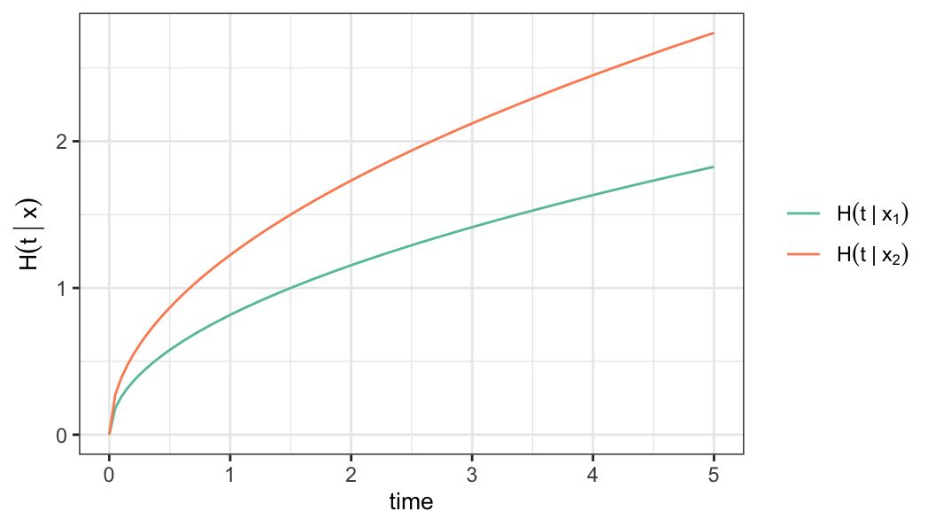
• Under proportional hazards model, the cumulative hazard function is defined as \[ \begin{aligned} H(t\,\vert\,\mathbf{x})&=\int_0^t h(u\,\vert\,\mathbf{x})du \notag \\[.2em] &= r(\mathbf{x}) \int_0^t h_0(u)du\notag\\[.2em] &=r(\mathbf{x})H_0(t) \end{aligned} \]

---

• Under proportional hazards model, the survivor function is defined as \[ \begin{aligned} S(t\,\vert\,\mathbf{x})&=e^{-H(t\,\vert\,\mathbf{x})} = e^{-r(\mathbf{x})H_0(t)} = \Big[S_0(t)\Big]^{r(\mathbf{x})} \end{aligned} \]

  • \(S_0(t)\,\rightarrow\) baseline survivor function and \(r(\mathbf{x})>0\)

  • Interpret the survival probabilities for the following cases \[(a) \;r(\mathbf{x})>1\quad \text{and} \quad(b)\; r(\mathbf{x})<1\]

---

Under proporitonal hazards model, comparison between baseline survivor function \(S_0(t)\) and \(S_1(t\,\vert\, x) = [S_0(t)]^{0.5}\)

---

Under proporitonal hazards model, comparison between baseline survivor function \(S_0(t)\) and \(S_1(t\,\vert\, x) = [S_0(t)]^{1.5}\)

---

Under proporitonal hazards model, comparison between hazard functions \(H(t\,\vert\,x_1)\) and \(H(t\,\vert\,x_2)=1.5H(t\,\vert\,x_1)\)

Parametric proportional hazards model

• Depending on whether the baseline hazard function \(h_0(t)\) is fully parametric or not, a PH model \(h(t\,\vert\,\mathbf{x})=h_0(t)r(\mathbf{x})\) could be either parametric or semi-parametric

  • PH model is parametric if \(h_0(t)=h_1(\boldsymbol{\alpha}, t)\) for some parameter vector \(\boldsymbol{\alpha}\)

  • PH model is semi-parametric if \(h_0(t)\) is unspecified

---

• Weibull model can be defined as both AFT and PH model

Weibull regression model

• Weibull as an AFT model \[ \begin{aligned} S(t\,\vert\,\mathbf{x}) &= \exp\Big(-[t/\alpha(\mathbf{x})]^{\delta}\Big) \end{aligned} \] where \[ \begin{aligned} \alpha(\mathbf{x}) & = \exp\big(\mathbf{x}'\boldsymbol{\beta}_{\sf AFT}\big) %\\ %u(\mathbf{x}) & = \mathbf{x}'\boldsymbol{\beta}_{\sf AFT} \end{aligned} \tag{6.5}\]

---

• Weibull as a PH model \[ \begin{aligned} h(t\,\vert\,\mathbf{x}) & = \frac{\delta}{\alpha(\mathbf{x})}\bigg[\frac{t}{\alpha(\mathbf{x})}\bigg]^{\delta-1} \\[.2em] & = (\delta t^{\delta-1})[\alpha(\mathbf{x})]^{-\delta}\\[.2em] &=h_1(\delta, t)\, r(\mathbf{x}) \end{aligned} \]

  • Assume \[ \begin{aligned} r(\mathbf{x}) =\exp\big(\mathbf{x}'\boldsymbol{\beta}_{\sf PH}\big) &= [\alpha(\mathbf{x})]^{-\delta} \\ \Rightarrow\;\exp\big(-\mathbf{x}'\boldsymbol{\beta}_{\sf PH}/\delta\big) & = \alpha(\mathbf{x}) \end{aligned} \tag{6.6}\]

---

• Equating the expression of \(\alpha(\mathbf{x})\) from the AFT (Equation 6.5) and PH (Equation 6.6) Weibull model, we can show \[ \begin{aligned} \exp\big(-\mathbf{x}'\boldsymbol{\beta}_{\sf PH}/\delta\big) & = \alpha(\mathbf{x}) = \exp\big(\mathbf{x}'\boldsymbol{\beta}_{\sf AFT}\big)\\[.25em] \Rightarrow\;\;\boldsymbol{\beta}_{\sf PH}&=-\delta\boldsymbol{\beta}_{\sf AFT} = -\frac{1}{b}\boldsymbol{\beta}_{\sf AFT} \end{aligned} \]

AFT and PH model

• Survivor function for some constants \(c>0\) and \(r(\mathbf{x})>0\) \[ \begin{aligned} S(t\,\vert\,\mathbf{x}_2) & = S(c\,t\,\vert\,\mathbf{x}_1) \\ S(t\,\vert\,\mathbf{x}_2) & = \big[S(t\,\vert\,\mathbf{x}_1)\big]^{r(\mathbf{x}_1)/r(\mathbf{x}_2)} \\ H(t\,\vert\,\mathbf{x}_2) & = \big[{r(\mathbf{x}_2)/r(\mathbf{x}_1)}\big]\,H(t\,\vert\,\mathbf{x}_1) \end{aligned} \]

6.2 Inference for Log-location-scale AFT Models

Likelihood methods

• Data \[ \big\{(y_i, \delta_i, \mathbf{x}_i), i=1, \ldots, n\big\} \]

  • Log-lifetime or log-censoring \(y_i=\log t_i\)

  • Censoring indicator \(\delta_i=I(\text{ith observation is a failure})\)

  • \(\mathbf{x}_i=(1, x_{i1}, \ldots, x_{ip})'\) is a vecor of covariates

---

• Assume \(Y_i\) follows a location-scale distribution with location parameter \(u(\mathbf{x}_i; \boldsymbol{\beta})\) and scale parameter \(b\)

• Regression model \[ \begin{aligned} u(\mathbf{x}_i; \boldsymbol{\beta}) &= \beta_0 + \beta_1x_{i1} + \cdots + \beta_{p}x_{ip} = \mathbf{x}_i'\boldsymbol{\beta} \end{aligned} \]

  • Vector of regression parameters \[\boldsymbol{\beta}=(\beta_0, \beta_1, \ldots, \beta_{p})'\]

  • Covariate vector \(\mathbf{x}_i\) contains both categorical and quantitative variables, and for accurate computation, quantitative variables are centered

---

The log-likelihood function \[ \ell(\boldsymbol{\beta}, b) = -r\log b \sum_{i=1}^n\big[\delta_i\log f_0(z_i) + (1-\delta_i)\log S_0(z_i)\big] \tag{6.7}\]

• \(r = \sum_{i=1}^n\delta_i\)

• \(z_i=\frac{y_i-u(\mathbf{x}_i; \boldsymbol{\beta})}{b}\)

• \(u(\mathbf{x}_i; \boldsymbol{\beta}) = \mathbf{x}_i'\boldsymbol{\beta}\)

---

Score functions

Elements of \((p+2)\)-dimensional vector of score function \[ \begin{aligned} U_j(\boldsymbol{\beta}, b) & = \frac{\partial \ell(\boldsymbol{\beta}, b)}{\partial \beta_j},\;j=0, 1, \ldots, p \\[.25em] U_b(\boldsymbol{\beta}, b)& = \frac{\partial \ell(\boldsymbol{\beta}, b)}{\partial b} \end{aligned} \]

• Homework: Obtain the expressions of score function (Eq. 6.3.3 and 6.3.4 of textbook)

---

Information matrix

Elements of observed information matrix \[ I(\boldsymbol{\beta}, b)=-\left[\begin{array}{cc} \frac{\partial^2 \ell}{\partial \boldsymbol{\beta} \partial \boldsymbol{\beta}^{\prime}} & \frac{\partial^2 \ell}{\partial \boldsymbol{\beta} \partial b} \\ \frac{\partial^2 \ell}{\partial b \partial \boldsymbol{\beta}^{\prime}} & \frac{\partial^2 \ell}{\partial b^2} \end{array}\right] \]

• Homework: Obtain the expressions of information matrix (Eq. 6.3.5, 6.3.6 and 6.3.7 of textbook)

---

MLEs

\[\begin{aligned} (\hat{\boldsymbol{\beta}}', \hat{b})' = {\arg \, \max}_{(\boldsymbol{\beta}', b)' \in\, \Theta}\,\ell(\boldsymbol{\beta}, b) \end{aligned}\]

• Iterative procedures (e.g. Newton-Raphson method) is used obtain MLE for \(\boldsymbol{\beta}\) and \(b\)

• MLEs \((\hat{\boldsymbol{\beta}}', \hat{b})'\) follow a \((p+2)\)-variate normal distribution with mean \(({\boldsymbol{\beta}}', {b})'\) and variance matrix \[\begin{aligned} \hat{V} = \big[I(\hat{\boldsymbol{\beta}}, \hat{b})\big]^{-1} \end{aligned}\]

• Large sample based tests and confidence intervals can be obtained using the sampling distribution of \((\hat{\boldsymbol{\beta}}', \hat{b})'\)

Test of hypothesis

Let \(\boldsymbol{\beta}' = (\boldsymbol{\beta}_1', \boldsymbol{\beta}_2')\), where \(\boldsymbol{\beta}_1\) is a \(k\)-dimensional vector of regression parameters, where \(k<p\) \[\begin{aligned} H_0: \boldsymbol{\beta}_1 = \boldsymbol{\beta}_1^0 \end{aligned}\]

• Likelihood ratio test statistic \[\begin{aligned} \Lambda_1 = 2\ell(\hat{\boldsymbol{\beta}}_1, \hat{\boldsymbol{\beta}}_2, \hat b) - 2\ell(\boldsymbol{\beta}_1^0, \tilde{\beta}_2, \tilde b)\label{LRT-AFT} \end{aligned}\]

  • \((\tilde{\boldsymbol{\beta}}', \tilde{b})' = {\arg\,\max}_{(\boldsymbol{\beta}_2', b)' \in\, \Theta}\,\ell(\boldsymbol{\beta}_1^0, \boldsymbol{\beta}_2, b)\)

  • Under \(H_0\), \(\Lambda_1\sim\chi^2_{(k)}\)

---

Let \(\boldsymbol{\beta}' = (\boldsymbol{\beta}_1', \boldsymbol{\beta}_2')\), where \(\boldsymbol{\beta}_1\) is a \(k\)-dimensional vector of regression parameters, where \(k<p\) \[\begin{aligned} H_0: \boldsymbol{\beta}_1 = \boldsymbol{\beta}_1^0 \end{aligned}\]

• Wald statistic \[\begin{aligned} \Lambda_2 = (\boldsymbol{\beta}_1 - \boldsymbol{\beta}_1^0)'V_{11}^{-1}(\boldsymbol{\beta}_1 - \boldsymbol{\beta}_1^0)\label{wald-AFT} \end{aligned}\]

  • \(V_{11}=var(\hat{\boldsymbol{\beta}}_1)\) is a \(k\times k\) matrix and \[\begin{aligned} \hat{V} = \big[I(\hat{\boldsymbol{\beta}}, \hat{b})\big]^{-1} = \begin{bmatrix}V_{11} &V_{12} \\ V_{12}' & V_{22}\end{bmatrix} \end{aligned}\]

    • Under \(H_0\), \(\Lambda_1\sim\chi^2_{(k)}\)

---

Null hypothesis \[\begin{aligned} H_0: \beta_j=0 \end{aligned}\]

• Test statistic \[\begin{aligned} Z_j = \frac{\hat\beta_j}{se(\hat\beta_j)} \end{aligned}\]

• \(100(1-\alpha)\%\) confidence interval for \(\beta_j\) \[ \hat\beta_j \pm z_{1-\alpha/2}\,se(\hat\beta_j) \]

• For a small sample, LRT statistic can be used to test the hypothesis and to obtain confidence interval

Quantiles

• The \(pth\) quantile of \(Y\) given \(\mathbf{x}\) \[\begin{aligned} y_p(\mathbf{x}) = \mathbf{x}'\boldsymbol{\beta} + bw_p \end{aligned}\]

• Estimate and corresponding SEs of \(pth\) quantile
  \[ \begin{aligned} \hat y_p(\mathbf{x}) &= \mathbf{x}'\hat{\boldsymbol{\beta}} + \hat{b}w_p\\[.2em] \text{and using delta method}, \quad se\big(\hat y_p(\mathbf{x})\big) &=\mathbf{a}'V\mathbf{a} \end{aligned} \]

  • \(\mathbf{a} = (\mathbf{x}', w_p)\) and \(w_p=S_0^{-1}(1-p)\)

• \(100(1-\alpha)\%\) confidence interval for \(y_p\) \[ \hat y_p \pm z_{1-\alpha/2}\,se\big(\hat y_p(\mathbf{x})\big) \]

Survival probability

• We are interest to obtain confidence interval for \(S(y_0)\), which can be expressed in terms of the parameters of location-scale distribution as \[\begin{aligned} S(y_0) &= S_0\Big(\frac{y_0 - \mathbf{x}'\boldsymbol{\beta}}{b}\Big)\\[.2em] S_0^{-1}\big(S(y_0)\big) & = \frac{y_0 - \mathbf{x}'\boldsymbol{\beta}}{b} = \psi(\mathbf{x}) \end{aligned}\]

---

• Estimate and the corresponding SE of \(\psi(\mathbf{x})\) \[ \begin{aligned} \hat\psi(\mathbf{x}) = \frac{y_0 - \mathbf{x}'\hat{\boldsymbol{\beta}}}{\hat b}\;\;\text{and using delta method,}\;\; se\big(\hat\psi(\mathbf{x})\big) = [\mathbf{a}'V\mathbf{a}]^{1/2} \end{aligned} \]

  • \(\mathbf{a}' = ({-1}/{\hat b})\big(\mathbf{x}', \hat\psi(\mathbf{x})\big)\)

• \((1-\alpha)100\%\) confidence interval for \(\psi(\mathbf{x})\) \[ \hat\psi(\mathbf{x}) \pm z_{1-\alpha/2}\,se\big(\hat\psi(\mathbf{x})\big) \]

---

• Wald-type \((1-\alpha)100\%\) confidence interval for \(S(y_0)\) \[\begin{aligned} \hat\psi(\mathbf{x}) - z_{1-\alpha/2}\,se\big(\hat\psi(\mathbf{x})\big) & <\psi(\mathbf{x}) < \hat \psi(\mathbf{x}) + z_{1-\alpha/2}\,se\big(\hat\psi(\mathbf{x})\big) \\[.2em] L & <\psi(\mathbf{x}) < U \\[.2em] L &<S_0^{-1}\big(S(y_0)\big) < U \\[.2em] S_0(L) & < S(y_0) < S_0(U) \end{aligned}\]

6.3 Weibull AFT

• Distributional assumption \[\begin{align*} T(\mathbf{x}) = (T\,\vert\,\mathbf{x})&\sim\text{Weib}\big(\alpha(\mathbf{x}), \delta\big)\\[.25em] Y(\mathbf{x})=(Y\,\vert\,\mathbf{x})=(\log T\,\vert\,\mathbf{x})&\sim\text{EV}\big(u(\mathbf{x}), b\big) \end{align*}\]

• Regression model for the parameters \[\begin{align*} u(\mathbf{x}) & = \beta_0 + \beta_1 x_1 + \cdots + \beta_px_p =\mathbf{x}'\boldsymbol{\beta}\\ \alpha(\mathbf{x}) & = \exp\big(\mathbf{x}'\boldsymbol{\beta}\big) \end{align*}\]

  • \(\mathbf{x} = (1, x_1, \ldots, x_p)'\)

  • \(\boldsymbol{\beta} = (\beta_0, \beta_1, \ldots, \beta_p)'\)

---

• Regression model for the response \[\begin{align*} Y(\mathbf{x}) & = \mathbf{x}'\boldsymbol{\beta} + bZ \end{align*}\]

  • \(Z\sim \text{EV}(0, 1)\)

  • \(f_0(z) = \exp(z- e^z)\)

  • \(S_0(z) = \exp(-e^z)\)

---

• Log-likelihood function \[\begin{align*} \ell(\boldsymbol{\beta}, b) & = -r\log b +\sum_{i=1}^n\Big[\delta_i\log f_0(z_i) + (1-\delta_i)\log S_0(z_i)\Big]\\[.25em] &=-r\log b + \sum_{i=1}^n (\delta_i z_i-e^{z_i}) \end{align*}\]
  • \(z_i=(y_i - \mathbf{x}_i'\boldsymbol{\beta})/b\)
• We can now obtain score functions, information matrix, and MLE’s for \(\beta\) and \(b\) (according to Section 6.2.)

---

• We’ve already seen that the Weibull model implies a proportional hazard model

• It is the only parametric model that is both an AFT model and a Proportional Hazards (PH) model at the same time

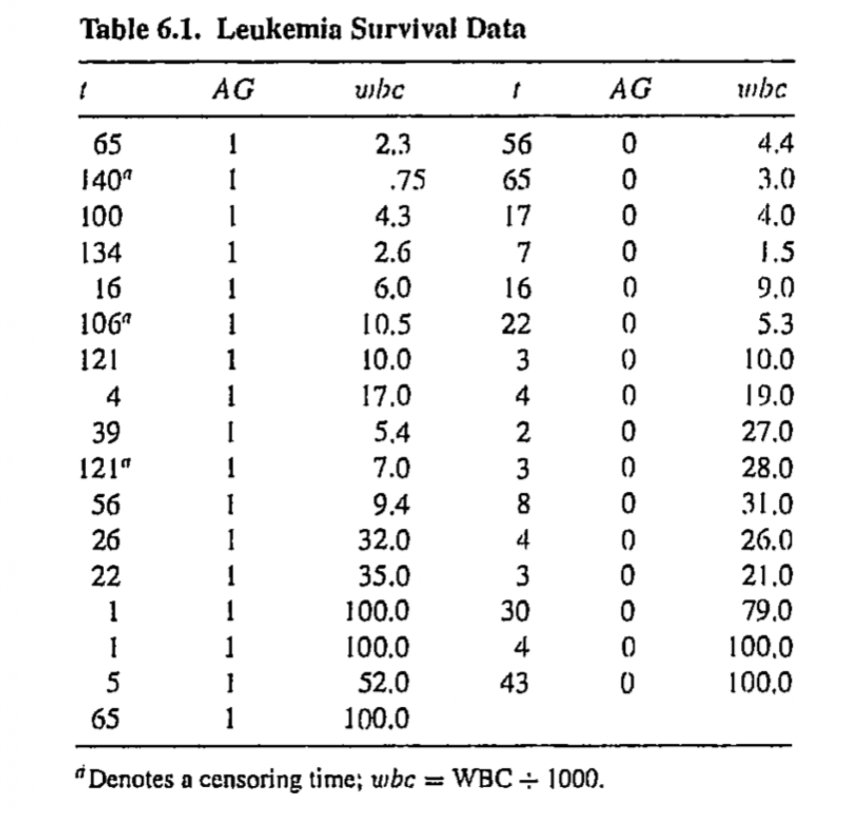
Leukemia survival times

• Data on survival times for 33 leukemia patients are available, where survival times are in weeks from diagnosis

• Data on two covariates are also available

  • White blood cell count (WBC) at diagnosis

  • Binary variable AG indicates a positive (AG=1) or negative (AG=0) test related to white blood cell characteristics

---

---

tab6_1

# A tibble: 33 × 5
    time   wbc    AG status   lwbc
   <dbl> <dbl> <int>  <dbl>  <dbl>
 1    65  2.3      1      1  0.833
 2   140  0.75     1      0 -0.288
 3   100  4.3      1      1  1.46 
 4   134  2.6      1      1  0.956
 5    16  6        1      1  1.79 
 6   106 10.5      1      0  2.35 
 7   121 10        1      1  2.30 
 8     4 17        1      1  2.83 
 9    39  5.4      1      1  1.69 
10   121  7        1      0  1.95 
# ℹ 23 more rows

---

• Consider Weibull AFT model with covariates \(x_1=AG\) and \(x_2=\log(wbc)\) \[\begin{aligned} Y = \beta_0 + \beta_1 x_1 + \beta_2x_2 +bZ \end{aligned} \tag{6.8}\]

  • \(Z\sim \text{EV}(0, 1)\)

---

Fit Weibull regression model Equation 6.8 using R

mod62 <- survreg(Surv(time, status) ~ AG + lwbc, 
                 data = tab6_1, dist = "weibull")

mod62E <- survreg(Surv(log(time), status) ~ AG + lwbc, 
                 data = tab6_1, dist = "extreme")

---

MLEs of model parameters

tidy(mod62, conf.int = T) |> 
  mutate(p.value = scales::pvalue(p.value))

# A tibble: 4 × 7
  term        estimate std.error statistic p.value conf.low conf.high
  <chr>          <dbl>     <dbl>     <dbl> <chr>      <dbl>     <dbl>
1 (Intercept)    3.84      0.534     7.19  <0.001     2.79     4.89  
2 AG             1.18      0.427     2.76  0.006      0.340    2.01  
3 lwbc          -0.366     0.150    -2.45  0.014     -0.660   -0.0731
4 Log(scale)     0.112     0.147     0.765 0.444     NA       NA     

---

Fitted model with \(x_1=AG\) and \(x_2=\log(wbc)\)

\[ \hat Y = 3.841 + 1.177 x_1 -0.366 x_2 + \exp\big({1.119}\big) Z \]

---

• Variance matrix of the estimated parameters

vcov(mod62) %>% round(3)

            (Intercept)     AG   lwbc Log(scale)
(Intercept)       0.286 -0.130 -0.067      0.003
AG               -0.130  0.182  0.016      0.005
lwbc             -0.067  0.016  0.022     -0.005
Log(scale)        0.003  0.005 -0.005      0.021

---

Summary of Weibull AFT model fit

term	estimate	std.error	statistic	p.value	conf.low	conf.high
\(\beta_0\)	3.841	0.534	7.188	<0.001	2.794	4.889
\(\beta_1\)	1.177	0.427	2.757	0.006	0.340	2.014
\(\beta_2\)	-0.366	0.150	-2.449	0.014	-0.660	-0.073
\(\log b\)	0.112	0.147	0.765	0.444	NA	NA

• AG and WBC have significant effects on leukemia survival times. Positive AG and low WBC count are associated with more prolonged survival

• Since \(\log b\) is not significant, i.e. there is not enough evidence to reject \(H_0: \log b=1\), exponential AFT model would be appropriate for analyzing this data

---

Interpretations

\[\begin{align*} \exp(\hat\beta_1) = \exp(1.177) = 3.246 \end{align*}\]

• A specific quantile (say median) lifetime of a patient with a positive AG value (i.e. \(x_1=1\)) is 3.2 times that of a patient with a negative AG (i.e. \(x_1=0\)) value provided WBC value remains constant

• Note this interpretation is true for any quantile (Why?)

---

\[ \begin{aligned} \exp(\hat\beta_2) = \exp(-0.366) = 0.693 \end{aligned} \]

• A specific quantile (say median) lifetime of a patient decreases 30.7 percent with one unit increase of log(WBC) [or 2718 unit increase of true WBC count] provided AG value remains constant

---

Fitted values

augment(mod62, type.predict = "response") |> 
  select(1:4) |> 
  slice(1:3)

# A tibble: 3 × 4
  `Surv(time, status)`    AG   lwbc .fitted
                <Surv> <int>  <dbl>   <dbl>
1                  65      1  0.833   111. 
2                 140+     1 -0.288   168. 
3                 100      1  1.46     88.6

---

augment(mod62, type.predict = "link") |> 
  mutate(.fittedE = exp(.fitted)) |> 
  select(2:4, .fittedE) |> 
  slice(1:3)

# A tibble: 3 × 4
     AG   lwbc .fitted .fittedE
  <int>  <dbl>   <dbl>    <dbl>
1     1  0.833    4.71    111. 
2     1 -0.288    5.12    168. 
3     1  1.46     4.48     88.6

• Estimate for a subject with \(AG=1\) and \(\log(wbc) = .833\)

\[ \hat u = \hat\beta_0 + \hat\beta_1 (1) + \hat\beta_2 (.833) = (3.841) + (1.177)(1) + (-0.366)(.833) = 4.713 \]

---

#predict(object = mod62, newdata = tibble(AG = 1, lwbc = .833), 
#        predict = "response")
augment(x = mod62, newdata = tibble(AG = 1, lwbc = .833), 
        type.predict = "response")

# A tibble: 1 × 4
     AG  lwbc .fitted .se.fit
  <dbl> <dbl>   <dbl>   <dbl>
1     1 0.833    111.    41.3

• Estimate for a subject with \(AG=1\) and \(\log(wbc) = .833\)

\[ \begin{aligned} \hat \alpha = \exp\big(\hat\beta_0 + \hat\beta_1 (1) + \hat\beta_2 (.833)\big) &= \exp\big((3.841) + (1.177)(1) + (-0.366)(.833)\big) \\&= \exp\big(4.713\big) = 111.399\end{aligned} \]

---

LRT

• Likelihood ratio tests for \(H_0: \beta_1=0\) \[\begin{align*} \Lambda_1(0) = 2\ell(\hat\beta_0, \hat\beta_1, \hat\beta_2, \log\hat b)-2\ell(\tilde\beta_0, 0, \tilde\beta_2, \log\tilde b) \end{align*}\]

  • \(\Lambda_1(0)\sim\chi^2_{(1)}\)

• The corresponding \(Z\) statistic \[ Z = \text{sign}({\hat\beta_1})\Lambda_1^{1/2}\sim \mathcal{N}(0, 1) \]

---

Estimate of model parameters under \(H_0: \beta_1=0\)

# mod62a <- update(mod62, formula = . ~ . - AG)
mod62a <- survreg(Surv(time, status) ~  lwbc, 
                 data = tab6_1, dist = "weibull")
tidy(mod62a)

# A tibble: 3 × 5
  term        estimate std.error statistic  p.value
  <chr>          <dbl>     <dbl>     <dbl>    <dbl>
1 (Intercept)    4.85      0.500      9.71 2.67e-22
2 lwbc          -0.500     0.165     -3.03 2.41e- 3
3 Log(scale)     0.222     0.146      1.52 1.28e- 1

---

LRTa <- anova(mod62a, mod62)

Terms	Resid. Df	-2*LL	Df	Deviance	Pr(>Chi)
lwbc	30	271.931	NA	NA	NA
AG + lwbc	29	265.013	1	6.918	0.009

• \(\Lambda_1(0) = 6.918\;\;\Rightarrow\;\; Z = 2.63\)

---

Comparison between Wald- and LRT-type Z statistics

term	estimate	Wald	LRT
\(\beta_0\)	3.841	7.188	NA
\(\beta_1\)	1.177	2.757	2.63
\(\beta_2\)	-0.366	-2.449	-2.46
\(\log b\)	0.112	0.765	NA

---

Quantiles

\[ \hat y_p = \mathbf{x}'\hat{\boldsymbol{\beta}} + \log(-\log(1-p))\,\hat b \]

• Consider a subject with covariate values \(x_1=1\) and \(x_2 =\log(10)\), the linear predictor \(\mathbf{x}'\hat{\boldsymbol{\beta}}\) \[\begin{align*} \hat u = \pmb{x}'\hat{\boldsymbol{\beta}} &= \hat\beta_0 +\hat\beta_1 + \log (10)\hat\beta_2 = 4.175 \end{align*}\]

---

• Median survival time of the patient with covariate values \(x_1=1\) and \(x_2 =\log(10)\) \[\begin{align*} \hat y_{.50} & = 4.175 + (-0.367)(1.119) = 3.765 \\ \hat t_{.50} & = \exp(3.765) = 43.163 \;\;\text{weeks} \end{align*}\]

• Homework: Obtain a 95% confidence interval of the median survival time of a patient with covariate values \(x_1=1\) and \(x_2=\log(10)\)

---

Survival probability

\[ S(y_0) = \exp\big\{-\exp\big[\big(y_0 - \mathbf{x}'\hat{\boldsymbol{\beta}}\big)/\hat b\big]\big\} \] For a patient with covariate values \(x_1=1\) and \(x_2=\log(10)\), obtain \(S(\log 10)\) \[ S(\log 10) = \exp\big\{-\exp\big[\big(\log 10 - 4.175)/1.119\big]\big\} = 0.816 \]

• Homework: Obtain the 95% CI for \(S(\log 10)\)

6.4 Log-normal AFT

• Distributional assumption \[\begin{align*} T(\mathbf{x}) = (T\,\vert\,\mathbf{x})&\sim\text{log-Norm}\big(\mu(\mathbf{x}), \sigma^2\big)\\[.25em] Y(\mathbf{x})=(Y\,\vert\,\mathbf{x})=(\log T\,\vert\,\mathbf{x})&\sim\mathcal{N}\big(\mu(\mathbf{x}), \sigma^2\big) \end{align*}\]

---

• Regression model for the parameters \[\begin{align*} \mu(\mathbf{x}) & = \beta_0 + \beta_1 x_1 + \cdots + \beta_px_p =\mathbf{x}'\boldsymbol{\beta} \end{align*}\]

• Regression model for the response \[\begin{align*} Y(\mathbf{x}) & = \mathbf{x}'\boldsymbol{\beta} + \sigma Z \end{align*}\]

  • \(Z\sim \mathcal{N}(0, 1)\)

  • \(f_0(z) = \phi(z)\)

  • \(S_0(z) = 1 - \Phi(z)\)

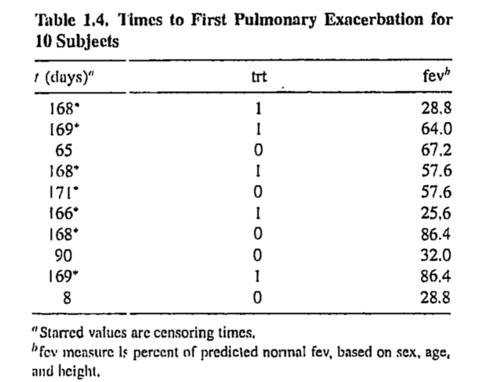
Times to pulmonary exacerbation

• Patients with cystic fibrosis are susceptible to an accumulation of mucus in the lungs, which leads to pulmonary exacerbation and deterioration of lung function

• A clinical trial was conducted to investigate the efficacy of the new drug DNase-1

  • Subjects are randomly assigned to a new treatment or a placebo

• Time of interest is the time to first exacerbation after randomization, and data on fev (forced expiratory volume at the time of randomization) are also measured

---

---

# A tibble: 761 × 13
      id   trt  time   fev  inst entry.dt   end.dt     ivstart ivstop time0
   <int> <int> <dbl> <dbl> <int> <date>     <date>       <dbl>  <dbl> <dbl>
 1     1     1   168  28.8     1 1992-03-20 1992-09-04      NA     NA   168
 2     2     1   169  64       1 1992-03-24 1992-09-09      NA     NA   169
 3     3     0    65  67.2     1 1992-03-24 1992-09-08      65     75   168
 4     4     1   168  57.6     1 1992-03-26 1992-09-10      NA     NA   168
 5     5     0   171  57.6     1 1992-03-24 1992-09-11      NA     NA   171
 6     6     1   166  25.6     1 1992-03-27 1992-09-09      NA     NA   166
 7     7     0   168  86.4     1 1992-03-27 1992-09-11      NA     NA   168
 8     8     0    90  32       1 1992-03-28 1992-09-10      90    104   166
 9     9     1   169  86.4     2 1992-02-27 1992-08-14      NA     NA   169
10    10     0     8  28.8     2 1992-03-06 1992-08-22       8     22   169
# ℹ 751 more rows
# ℹ 3 more variables: status <dbl>, fevm <dbl>, visit <int>

---

• Assume survival time \(T(\mathbf{x})\) follows a log-normal distribution with scale parameter \(\alpha(\mathbf{x})\) and shape parameter \(\delta\)

• Consider following AFT model for log survival time \[ Y(\mathbf{x}) = \beta_0 + \beta_1 x_1 + \beta_2 x_2 + \sigma Z \]

  • \(Z\sim\mathcal{N}(0, 1)\)

  • \(x_1 = I(\text{trt}=1)\)

  • \(x_{2} = \text{fev} - \text{mean(fev)}\)

---

• R codes for fitting the AFT model

mod63a <- survreg(Surv(log(time), status) ~ trt + fevm, 
                  dist = "gaussian",
                  data = tab1_4) 

---

tidy(mod63a)

# A tibble: 4 × 5
  term        estimate std.error statistic  p.value
  <chr>          <dbl>     <dbl>     <dbl>    <dbl>
1 (Intercept)   5.09     0.0684      74.4  0       
2 trt           0.336    0.0951       3.53 4.19e- 4
3 fevm          0.0159   0.00197      8.09 5.91e-16
4 Log(scale)    0.137    0.0408       3.36 7.84e- 4

---

• AFT model \[\begin{align*} Y & = \mathbf{x}'\boldsymbol{\beta} + bZ\;\;\Rightarrow\;\;T =\exp(\mathbf{x}'\boldsymbol{\beta})\exp(bZ) \end{align*}\]

  • \(\mathbf{x}'\boldsymbol{\beta}=\beta_0 + \beta_1x_1 + \cdots + \beta_px_p\)

• For a binary predictor \(x_j\) \[ T =\exp(\mathbf{x}'\boldsymbol{\beta})\exp(bZ) = \begin{cases} \exp(bZ) & \text{for control} \\ \exp(\beta_j)\exp(bZ) &\text{for treatment} \end{cases} \]

• It can be shown that \[ T_{trt} = \exp(\beta)\;T_{control} \]

---

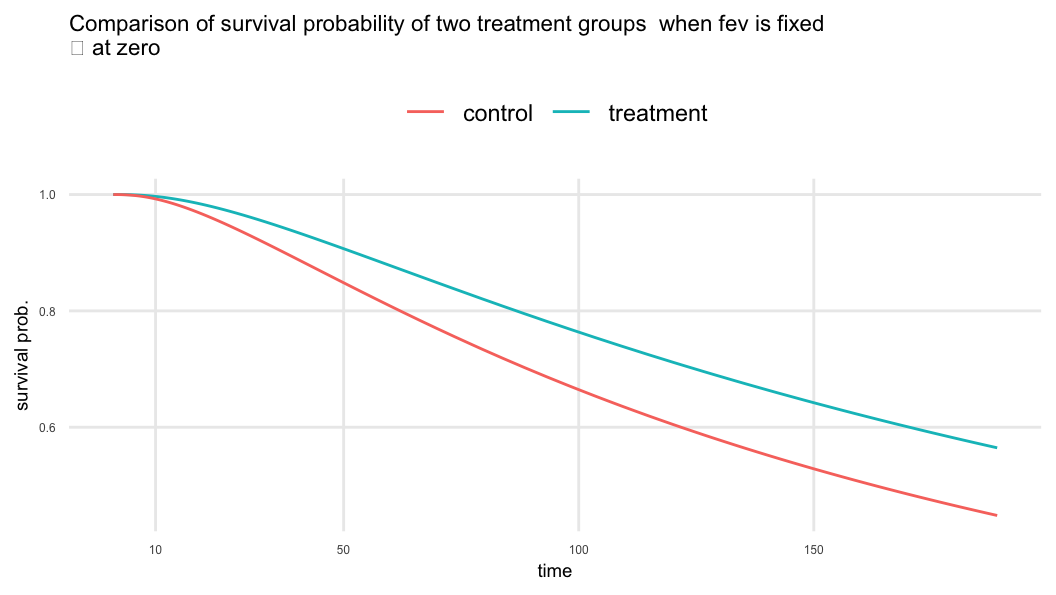
• \(\beta_{trt}=0.336 \;\; \Rightarrow\;\; \exp(\beta_{trt}) = 1.399\)

  • Treatment increases the time to first pulmonary exacerbation by about 40% compared to the control when fev is fixed

• \(\beta_{fev}=0.016 \;\; \Rightarrow\;\; \exp(\beta_{fev}) = 1.016\)

  • One-unit increase in fev results about 2% increase in lifetime provided treatment is constant

---

6.5 Log-logistic AFT

• Distributional assumptions \[\begin{align*} T(\mathbf{x}) = (T\,\vert\,\mathbf{x})&\sim\text{log-logistic}\big(\alpha(\mathbf{x}), \beta\big)\\[.25em] Y(\mathbf{x})=(Y\,\vert\,\mathbf{x})=(\log T\,\vert\,\mathbf{x})&\sim\text{logistic}\big(u(\mathbf{x}), b\big) \end{align*}\]

---

• Regression model for the parameters \[\begin{align*} u(\mathbf{x}) & = \beta_0 + \beta_1 x_1 + \cdots + \beta_p x_p =\mathbf{x}'\boldsymbol{\beta} \\ \alpha(\mathbf{x}) & = e^{u(\mathbf{x})} \end{align*}\]

• Regression model for the response \[\begin{align*} Y(\mathbf{x}) & = \mathbf{x}'\boldsymbol{\beta} + bZ \end{align*}\]

  • \(Z\sim \text{Logistic}(0, 1)\)

  • \(f_0(z) = e^{z}[1 + e^z]^{-2}\)

  • \(S_0(z) = [1 + e^z]^{-1}\)

---

• Lifetime distribution \[T(\pmb x) \sim \text{Log-Logistic}\big(\alpha(\pmb x), \delta\big)\]

• The survivor function \[S(t\,\vert\, \pmb x) = \frac{1}{1 + \big(t/\alpha(\pmb x)\big)^{\delta}}\;\Rightarrow\;\frac{1 - S(t\,\vert\, \pmb x)}{S(t\,\vert\, \pmb x)} = \big(t/\alpha(\pmb x)\big)^{\delta}\]

  • \(\big(t/\alpha(\pmb x)\big)^{\delta}\,\rightarrow\) the odds of failure at time \(t\) for a subject with covariate vector \(\pmb x\)

---

• For two subjects with covariate vectors \(\pmb x_1\) and \(\pmb x_2\) \[\frac{[1 - S(t\,\vert\, \pmb x_2)]/S(t\,\vert\, \pmb x_2)}{[1 - S(t\,\vert\, \pmb x_1)]/S(t\,\vert\, \pmb x_1)} = \bigg[\frac{\alpha(\pmb x_1)}{\alpha(\pmb x_2)}\bigg]^{\delta}, \;\;\text{independent of $t$}\]

• A model of the form \[\frac{1 - S(t\,\vert\, \pmb x)}{S(t\,\vert\, \pmb x)} = \big(t/\alpha(\pmb x)\big)^{\delta}\;\Rightarrow\;\log \frac{1 - S(t\,\vert\, \pmb x)}{S(t\,\vert\, \pmb x)} = \delta\log(t) - \delta\log \alpha(\pmb x)\] is known as the proportional odds model

---

• Consider a model \(\log \alpha(x) = \beta_0 + \beta_1 x\) \[\frac{[1 - S(t\,\vert\, x=1)]/S(t\,\vert\, x=1)}{[1 - S(t\,\vert\, x=0)]/S(t\,\vert\, x=0)} = e^{-\delta\beta_1} = e^{-\beta_1^{\star}}\]

  • The odds of failure at time \(t\) for a subject with \(x=1\) is \(\exp(-\beta^\star)\) times that of the odds of failure for a subject with \(x=0\)

Times to pulmonary exacerbation

• R codes for fitting AFT model

mod63b <- survreg(Surv(log(time), status) ~ trt + fevm, 
                  dist = "logistic",
                  data = tab1_4) 

---

tidy(mod63b)

# A tibble: 4 × 5
  term        estimate std.error statistic  p.value
  <chr>          <dbl>     <dbl>     <dbl>    <dbl>
1 (Intercept)   5.08     0.0600      84.6  0       
2 trt           0.293    0.0861       3.41 6.55e- 4
3 fevm          0.0145   0.00181      8.00 1.20e-15
4 Log(scale)   -0.489    0.0466     -10.5  8.08e-26

---

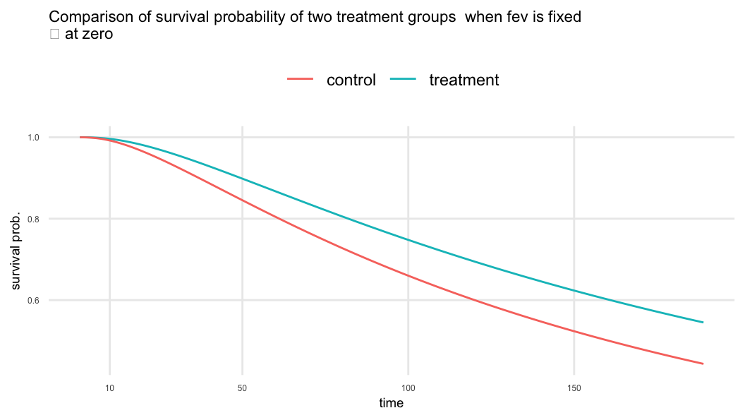
• \(\beta_{trt}=0.293 \;\; \Rightarrow\;\; \exp(\beta_{trt}) = 1.341\)

  • Treatment increases the time to first pulmonary exacerbation by about 34% compared to the control when fev is fixed

• \(\beta_{fev}=0.014 \;\; \Rightarrow\;\; \exp(\beta_{fev}) = 1.015\)

  • One-unit increase in fev results in a 1.5% increase in lifetime provided treatment is constant

---

• Interpret the treatment effect in terms of odds of failure \[ \frac{\big[1-S(t\,\vert\,trt=1, fev=x)\big]/S(t\,\vert\,trt=1, fev=x)}{\big[1-S(t\,\vert\,trt=0, fev=x)\big]/S(t\,\vert\,trt=0, fev=x)} = \exp(-\hat\delta\hat\beta_1) = 0.62 \]

  • \(\hat\delta = \exp(-\log \hat b) = \exp(0.489) = 1.631\)

  • The odds of failure is 38% lower in the treatment group compared to the control group provided fev value is fixed

---

---

Comparison between normal and logistic regression models in analysing time to pulmonary exacerbation data

term	est	se	est	se
(Intercept)	5.093	0.068	5.078	0.060
trt	0.336	0.095	0.293	0.086
fevm	0.016	0.002	0.014	0.002
Log(scale)	0.137	0.041	-0.489	0.047

Other regression models

• Additive hazards model \[h(t\,\vert\, \pmb{x}) = h_0(t; \alpha) + r(\pmb x; \pmb \beta)\]

6.6 Graphical methods and model assessment

• Graphical methods are helpful in summarizing information and suggesting possible models

• These methods also provide ways to check assumptions concerning the form of a lifetime distribution and its relationship to covariates

• Exploratory analysis of a lifetime distribution given covariates would helpful to select the appropiate Model for the analysis

---

• For a single quantitative covariate, a plot of lifetime or log-lifetime against the covariate or a function of it could indicate the nature of the relationship between lifetime and the covariate

• If the proportion of censoring is small, such a plot would be helpful, different symbols can be used in those plots for censored and failure times

• When more than one quantitative covariate and light censoring, one can consider grouping individuals so that within a group, individuals will have similar values of important covariates

• Let there are \(J\) such groups and \(\hat S_j\) is the Kaplan-Meier estimate for the group \(j=1, \ldots, J\)

---

AFT model \[ S(t\,\vert\,\mathbf{x}) = S_0\bigg[\frac{\log t - u(\mathbf{x})}{b}\bigg] \]

• If \(u(\mathbf{x})\) is approximately constant for individuals within each group \(j=1, \ldots, J\), and if an AFT model is appropriate, the plots of \[\log[-\log S(t\,\vert\, \mathbf{x})]\;\;\text{ vs}\;\; \log t\] should be roughly parallel in horizontal direction (\(\log t\))

---

Proportional hazards model \[ S(t\,\vert\,\mathbf{x}) = \big[S_0(t)\big]^{r(\mathbf{x})} \]

• If \(r(\mathbf{x})\) is approximately constant for individuals within each group \(j=1, \ldots, J\), and if a proportional hazards model is appropriate, the plots of \[\log[-\log S(t\,\vert\, \mathbf{x})]\quad\text{vs}\quad \log t\] should be roughly parallel in vertical direction

---

• If the plots of \(\log[-\log S(t\,\vert\, \mathbf{x})]\) vs \(\log t\) is roughly linear then Weibull models are suggested

• In addition to linear, if the plots are parallel, then Weibull models with a constant shape parameter are suggested, in that case, both AFT and PH models can be considered

• Statistical analysis of data is an iterative process involving exploration, model fitting, and model assessment

References

Collett, David. 2015. Modelling Survival Data in Medical Research. Chapman; Hall/CRC. https://doi.org/10.1201/b18041.

Cox, David R. 1972. “Regression Models and Life-Tables.” Journal of the Royal Statistical Society: Series B (Methodological) 34 (2): 187–202.